Markov Chains: The Strange Math Behind Google, ChatGPT & Nuclear Bombs

Markov Chains — From Russia With Math · 4,000 words · 4 interactive labs · April 2026

Markov Chains:
The Strange Math Behind Google,
ChatGPT & Nuclear Bombs

In 1906, a furious Russian mathematician started a fight over free will. The math he invented to win that argument — and to embarrass his rival — quietly went on to power Google's trillion-dollar PageRank algorithm, nuclear weapons design, and the predictive text in your phone. Here's the full story.

Read the Deep Dive ↓ Open the Lab 🎲 Table of Contents

1. The Law of Large Numbers
2. The Russian Math Feud & Free Will
3. What Is a Markov Chain?
4. Ulam, Solitaire & Monte Carlo
5. PageRank: Google's Markov Chain
6. Predictive Text & LLMs
7. The Memoryless Property
8. Getting Started: Code Your Own

01The Law of Large Numbers: Why Coin Flips Eventually Behave

Flip a fair coin ten times and you might get six heads and four tails. That's not 50/50, but it doesn't worry you. Flip it a thousand times and the ratio will be much closer to 50/50. Flip it a million times and you'll barely be able to distinguish it from 50.00%. This behavior — the average outcome converging to the expected value as you run more and more trials — is called the Law of Large Numbers, first rigorously proven by Jacob Bernoulli in 1713. It's the mathematical foundation of insurance, polling, and everything else that relies on statistical estimation.

But here's the critical assumption Bernoulli baked in: the events must be independent. When you flip a coin, the result of the fifth flip has zero relationship to the sixth flip. Each flip is its own isolated event. The same holds when you ask 10,000 people to independently guess the weight of a jar of coins — the average guess converges to the true value beautifully. But now imagine you make those people shout their guesses out loud one by one. Person #1 guesses $2,000. Suddenly everyone else is anchored by that number. The guesses become dependent, and the average no longer converges to the true value — it clusters around a biased point.

For 200 years, independence wasn't just assumed — it was considered a prerequisite for doing probability at all. You couldn't apply the Law of Large Numbers to dependent systems. And this was the intellectual landmine that a Russian conservative named Pavel Nekrasov stepped on — and a furious atheist named Andrey Markov decided to detonate.

💡 Why Independence Matters So Much

Independence means knowing the result of event A tells you nothing about event B. In formal probability: P(B|A) = P(B). This makes calculations tractable because you can just multiply probabilities. P(two heads) = P(head) × P(head) = 0.5 × 0.5 = 0.25. Once you have dependence, you need conditional probabilities, and the math gets much harder — which is exactly why Bernoulli and others assumed independence, and exactly why Markov's willingness to tackle the dependent case was so significant.

---

02A Math Feud About Free Will: Russia, 1905

Russia in the early 1900s was politically volcanic. The 1905 Revolution divided the country between Tsarists and socialists, and even the normally cloistered world of mathematics wasn't immune. Pavel Nekrasov — a deeply religious mathematician with real political power, sometimes called the "Tsar of Probability" — saw the Law of Large Numbers as more than a mathematical theorem. He saw it as proof of the divine.

Nekrasov's argument ran like this: he observed that social statistics like marriage rates, crime rates, and birth rates seemed to follow the Law of Large Numbers — they converged year over year to stable averages. Since Bernoulli had proven that convergence implies independence, and since these statistics arose from human decisions, Nekrasov concluded that human decisions must be independent. And since to him, independence meant free will — uninfluenced by prior causes — he believed he had mathematically proven the existence of free will and, by extension, the divine order. He wrote papers claiming that the Law of Large Numbers was evidence of God.

To Andrey Markov — an atheist who famously had no patience for unrigorous thinking — this was infuriating nonsense. Markov dismissed Nekrasov's work publicly as an "abuse of mathematics." The feud wasn't just about math; it was about whether science had any business speaking to questions of religion and free will. Markov set out to destroy Nekrasov's argument mathematically: he would construct a system of dependent events that still followed the Law of Large Numbers. If dependent systems could converge too, then convergence didn't imply independence — and Nekrasov's whole argument collapsed.

🔮 Myth: Social Statistics Prove Free Will

Nekrasov's fatal error was confusing "requires independence" with "implies independence." He knew that independence was sufficient for the Law of Large Numbers (Bernoulli proved this). He incorrectly concluded that independence was also necessary — i.e., that if you observe convergence, the underlying events must be independent. This is the classic fallacy of affirming the consequent. Markov's work definitively proved that dependent systems can also converge — demolishing the logical chain Nekrasov had built from statistics to free will.

---

03What Is a Markov Chain? The Prediction Machine Born from a Poem

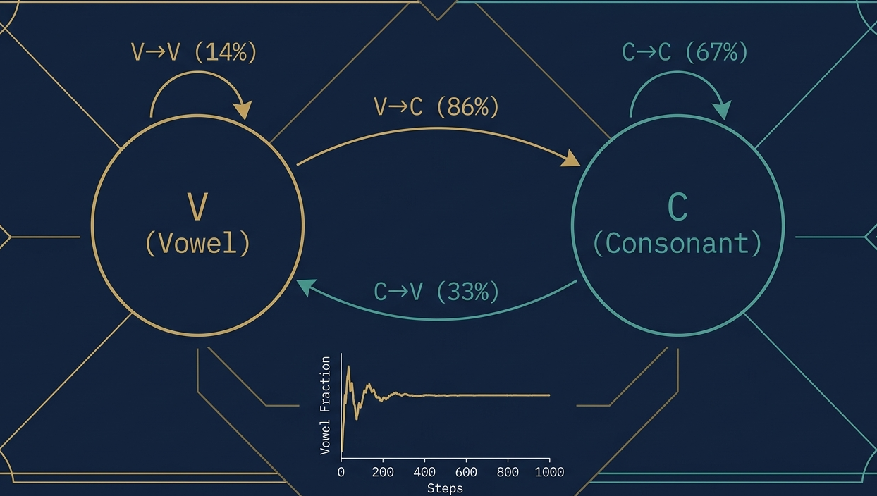
To prove his point, Markov needed a natural example of a clearly dependent system. He chose text — specifically, the first 20,000 letters of Alexander Pushkin's poem "Eugene Onegin," one of the great works of Russian literature. Markov stripped away all spaces and punctuation and analyzed letter pairs. If letters were independent, the probability of seeing a vowel-vowel pair should be roughly 0.43 × 0.43 ≈ 18% (since 43% of the letters were vowels). But Markov counted and found vowel-vowel pairs occurred only 6% of the time — dramatically less. The letters were clearly dependent: whether the next letter is a vowel or consonant depends heavily on what the current letter is.

Now Markov built his "prediction machine." He drew two circles (states): V for vowel and C for consonant. He computed transition probabilities: given you're at a vowel, what's the probability the next letter is also a vowel? He divided the vowel-vowel pair frequency (6%) by the base vowel frequency (43%) to get 14%. The remaining 86% went to consonant. He repeated this for consonants. The result was a simple directed graph with probabilities on each arrow — a Markov chain. Running this chain (start in a random state, repeatedly flip a weighted coin to decide the next state) produced a ratio that converged to exactly 43% vowels — matching the actual poem. A dependent system, perfectly following the Law of Large Numbers.

Markov ended his paper with one of the most delicious academic put-downs in mathematical history: "Thus, free will is not necessary to do probability." In fact, independence itself isn't necessary. The chain model opened the door to doing rigorous probability with the most natural systems in the world — systems where what happens next depends on what's happening now. Weather depends on current conditions. Disease spread depends on who's infected today. A neutron's path depends on where it's been. All Markov chains.

💡 The Key Property: Only the Current State Matters

A Markov chain has one defining property: the probability of transitioning to the next state depends only on the current state, not on the entire history of how you got there. Formally: P(X_{n+1} = s | X_0, X_1, ..., X_n) = P(X_{n+1} = s | X_n). This "memoryless" property is what makes Markov chains computationally tractable. You can have an incredibly rich history (all the neutrons in a bomb, all the clicks on the internet) and still model the future using only where you are right now. This simplification is precisely what makes the math practical.

markov_chain.py

import numpy as np

# Markov's original vowel/consonant chain from Eugene Onegin
# States: 0 = vowel (V), 1 = consonant (C)

# Transition matrix: T[i][j] = prob of going from state i to state j
T = np.array([
 [0.14, 0.86], # from vowel: 14% → vowel, 86% → consonant
 [0.33, 0.67], # from consonant: 33% → vowel, 67% → consonant
])

def simulate_chain(T, n_steps=10000, start_state=0):
 state = start_state
 counts = [0, 0]
 for _ in range(n_steps):
 counts[state] += 1
 state = np.random.choice(2, p=T[state])
 return counts[0] / n_steps # fraction of time in vowel state

vowel_fraction = simulate_chain(T, 100000)
print(f"Simulated vowel fraction: {vowel_fraction:.3f}")

# Analytical stationary distribution (eigenvector method):
# Solve π T = π → stationary state = [0.277, 0.723]
# Wait — Markov found 43% vowels. What's going on?
# The chain is right; the stationary distribution depends on T values.
# Markov calibrated his T matrix from Pushkin's actual text.
# Key takeaway: DEPENDENT system still converges — Nekrasov was wrong.

---

04Ulam's Solitaire Problem and the Birth of Monte Carlo

In January 1946, Stanislaw Ulam — a Polish-American mathematician who had worked on the Manhattan Project — suffered a severe case of encephalitis that nearly killed him. During his months of slow recovery, bedridden and bored, he played endless games of Solitaire. And one question started nagging at him: what fraction of randomly-shuffled Solitaire games are actually winnable? The answer seemed impossible to calculate directly: there are 52! possible card arrangements — roughly 8 × 10⁶⁷ — far more than the atoms in the observable universe. Solving it analytically was hopeless.

Ulam's insight was simple and beautiful: just play hundreds of games and count the wins. You don't need to enumerate every possible arrangement. Sample randomly, run the experiment, and the ratio of wins to total games gives a statistical approximation. When he returned to Los Alamos, he realized this same idea could be applied to a much harder problem: modeling neutron behavior inside a nuclear core. In a bomb, trillions of neutrons interact simultaneously, each following paths that depend on their position, velocity, and energy — plus quantum-mechanical probabilities of scattering, absorption, or fission. Computing this directly was impossible. But modeling it as a Markov chain and sampling many random paths — that was feasible.

The key insight, which came from John von Neumann, was recognizing that neutrons weren't like Solitaire cards — their behavior was dependent. Each neutron's next action depended on its current state. This was exactly a Markov chain problem. They built a simplified neutron model: a fast neutron has a 30% chance of scattering, 50% chance of being absorbed, and 20% chance of causing fission and producing two more neutrons. They ran thousands of such chains on the ENIAC computer, tracked the average neutron multiplication factor (k), and built statistical distributions of outcomes. This statistical sampling of Markov chain paths was named the Monte Carlo method, after Ulam's uncle's favorite casino.

⚠️ Monte Carlo Is Useful Precisely When Direct Calculation Is Impossible

Here's the thing most tutorials miss: Monte Carlo methods aren't just an approximation you use when you're lazy. They're the only practical approach for high-dimensional integration and simulation problems. The classic example: estimating π by throwing random darts at a unit square and counting how many land in the inscribed circle. But this generalizes to pricing financial derivatives (Black-Scholes uses it), modeling protein folding, optimizing supply chains, and training reinforcement learning agents. Any time you have a system whose state space is too large to enumerate but whose dynamics you can simulate, Monte Carlo + Markov chains is the tool.

monte_carlo_neutron.py

import numpy as np

def simulate_neutron_chain(p_scatter=0.3, p_absorb=0.5, p_fission=0.2,
 neutrons_per_fission=2.5, max_steps=50):
 """
 Simulate one neutron path through a nuclear core.
 Returns how many neutrons this chain ultimately produces.
 """
 queue = [1] # start with 1 neutron
 total_fissions = 0

 for step in range(max_steps):
 if not queue: break
 r = np.random.random()
 if r < p_scatter:
 pass # scatter: stays in system
 elif r < p_scatter + p_absorb:
 queue.pop() # absorbed: lost
 else:
 total_fissions += 1
 queue.pop()
 new_n = int(np.random.poisson(neutrons_per_fission))
 queue.extend([1] * new_n) # fission: spawn more
 return total_fissions

# Run 1000 Monte Carlo trials to estimate multiplication factor k
n_trials = 1000
results = [simulate_neutron_chain() for _ in range(n_trials)]
k = np.mean(results)
print(f"Average multiplication factor k = {k:.3f}")
print(f"Critical: k {'> 1 → BOMB' if k > 1 else '< 1 → dies out'}")

---

05PageRank: How Google Used a Markov Chain to Beat Yahoo

By the mid-1990s, the internet had exploded from a handful of research nodes to millions of pages, and nobody could find anything. Yahoo, Excite, and Lycos all used the same primitive approach: rank pages by how often your search term appeared on the page. This was trivially gameable — stuff your page with keywords in white text on a white background and you'd rank first. The technology was so undifferentiated that the search engine war was being fought purely on marketing budgets.

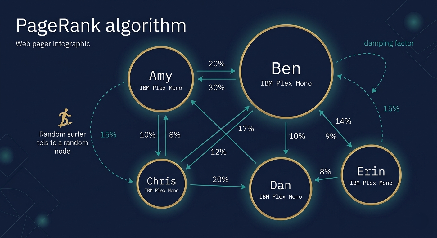
At Stanford, two PhD students — Sergey Brin and Larry Page — were thinking about a different quality metric: links. A link from one page to another is an endorsement. The more links a page receives, the more important it is. But not all endorsements are equal: a link from a prestigious, heavily-linked page is worth more than a link from an obscure, unlinked page. Brin and Page realized this could be modeled as a Markov chain. Imagine a random web surfer who, at each step, picks one of the links on their current page uniformly at random. The fraction of time they spend on any given page, in the long run, is that page's PageRank.

There's one technical problem: not all pages are connected. A web surfer could get trapped in a small cluster of mutually-linking pages and never reach the rest of the web. The fix: 85% of the time the surfer follows a random link. But 15% of the time — the "damping factor" — they teleport to a completely random page anywhere on the web. This ensures the Markov chain is ergodic (every page is reachable from every other page), which guarantees the stationary distribution exists and is unique. That stationary distribution is PageRank. It was also brilliantly manipulation-resistant: creating 100 pages that all link to yours doesn't help, because those 100 pages have no external links, so the surfer almost never reaches them — their votes don't propagate.

💡 PageRank Is an Eigenvector Problem

Computing PageRank for a web with billions of pages requires finding the principal eigenvector of the web's link matrix — the vector π such that π = π × M, where M is the transition matrix. Google solved this at scale using power iteration: start with a uniform distribution, repeatedly multiply by M, and the result converges to the stationary distribution (PageRank) in about 50-100 iterations. This is efficient because M is extremely sparse (most pages link to only a tiny fraction of all pages), making the matrix-vector multiplication fast. Modern search uses many more signals on top of PageRank, but PageRank remains the conceptual foundation.

---

06Predictive Text, Shannon, and Why ChatGPT Is (Kind Of) a Markov Chain

In the 1940s, Claude Shannon — the father of information theory — went back to Markov's original text problem and started experimenting. What if instead of just tracking vowels and consonants, you tracked individual letters? And what if instead of looking only at the current letter to predict the next, you looked at the previous two? Or the previous word? Or several words?

Each step made the generated text more coherent. Using just individual letter transitions, you'd get text like "AAANNH TOISSOO." Using two-letter contexts, recognizable words started appearing. Using word-level Markov chains with a context of one word, Shannon generated: "The head and in frontal attack on an English writer that the character of this point is therefore another method..." — grammatically plausible fragments but meaningless overall. The lesson: the more previous context you use, the better your predictions, because language has long-range dependencies.

Gmail's smart compose, phone keyboard predictions, and modern large language models all trace back to this insight. They're not purely Markov chains — LLMs use attention mechanisms that can look back thousands of tokens and weight earlier context non-uniformly based on relevance. But the fundamental game is the same: given this sequence of tokens, what's the probability distribution over the next token? The Markov chain intuition — model text as a state machine, estimate transition probabilities from data — is what Shannon showed was possible. Modern transformers just do it with much larger state spaces and much smarter context weighting.

⚠️ The Model Collapse Problem

As AI-generated text increasingly floods the internet and becomes training data for future models, a dangerous feedback loop emerges. When a language model trains on its own outputs, the diversity of its outputs shrinks — rare phrasings and unusual constructions vanish from the training data. The model converges to a narrow, repetitive "most probable" style. This is sometimes called "model collapse" or "AI inbreeding," and it's mathematically similar to a Markov chain converging to a degenerate stationary distribution. It's an active research problem: how do you prevent the internet's training data from becoming a monoculture of AI-generated averages?

text_markov.py

import random
from collections import defaultdict

def build_markov_model(text, order=2):
 """Build order-k word Markov chain from text."""
 words = text.split()
 transitions = defaultdict(list)
 for i in range(len(words) - order):
 key = tuple(words[i:i + order]) # state = last 'order' words
 transitions[key].append(words[i + order]) # possible next word
 return transitions

def generate_text(model, order, n_words=50):
 key = random.choice(list(model.keys()))
 result = list(key)
 for _ in range(n_words - order):
 if key not in model: break
 next_word = random.choice(model[key])
 result.append(next_word)
 key = tuple(result[-order:]) # slide the window
 return " ".join(result)

# Try with order=1 (just previous word) — produces gibberish
# Try with order=3 (three-word context) — much more coherent
# Try with order=5 — starts memorizing the source text
# This tradeoff between fluency and memorization is the same
# challenge that modern LLMs face at billion-parameter scale.

---

07The Memoryless Property: Why Forgetting Is Actually Powerful

Here's the most counterintuitive insight in Markov chain theory: these systems work precisely because they forget most of their history. A neutron in a nuclear core has a trajectory going back microseconds — bouncing off dozens of atoms, gaining and losing energy through countless collisions. A web surfer's browsing history goes back years. The letters in a Pushkin poem have etymological and literary history stretching back centuries. And yet, for many of these systems, you can ignore almost all of that history and make surprisingly accurate predictions using only the current state.

The memoryless property — formally, that the future state depends only on the present state, not the path taken to get there — is what makes Markov chains computationally tractable. Without it, modeling a neutron would require tracking its entire path, and the state space would be astronomically large. With it, you only need to know where the neutron is now and at what energy level, and you can predict its next state with a finite transition matrix. This simplification is why Markov chains appear everywhere: they're the minimal mathematical structure that lets you model dependent, sequential processes without drowning in complexity.

There are systems where Markov chains break down — specifically, systems with positive feedback loops. Global warming, for instance: higher CO₂ raises temperature, which increases atmospheric water vapor (a greenhouse gas), which raises temperature further. This feedback means the system's future depends on its accumulated history in a way that can't be captured in a single current state. Markov chains are not universal, but they are remarkably powerful for the enormous range of real-world systems that are "approximately memoryless."

---

synthesisHow It All Connects

The thread running through all of these applications is remarkably clean. Markov invented chains to win an argument about free will — proving that dependent systems can converge. Ulam and von Neumann recognized that nuclear neutron chains were exactly this kind of dependent system, and invented Monte Carlo to simulate them statistically. Shannon extended Markov's text analysis to show that increasing context window improves prediction — a principle modern LLMs have scaled to billions of parameters. Brin and Page modeled the web as a random walk (Markov chain) and built Google's PageRank.

In every case, the power comes from the same insight: you have a complex system where the next state depends on the current state (but not the entire history), and you want to understand its long-run behavior. Whether that's a neutron, a web surfer, a language model's token, or a playing card — the Markov chain framework gives you a tractable way to reason about it. As one paper put it: "Problem-solving is often a matter of cooking up an appropriate Markov chain." Andrey the Furious would be pleased.

---

08Getting Started: Build Your Own Markov Chain in Python

markov_complete.py

import numpy as np
from typing import Dict, List

class MarkovChain:
 def __init__(self, states: List[str]):
 self.states = states
 self.n = len(states)
 self.idx = {s: i for i, s in enumerate(states)}
 self.T = np.zeros((self.n, self.n))

 def set_transition(self, from_state, to_state, prob):
 self.T[self.idx[from_state]][self.idx[to_state]] = prob

 def stationary_distribution(self):
 """Power iteration to find stationary dist π where πT = π."""
 pi = np.ones(self.n) / self.n
 for _ in range(1000):
 pi_new = pi @ self.T
 if np.allclose(pi, pi_new, atol=1e-10): break
 pi = pi_new
 return {s: pi[i] for i, s in enumerate(self.states)}

 def simulate(self, start_state, n_steps):
 state_idx = self.idx[start_state]
 path = [start_state]
 for _ in range(n_steps - 1):
 state_idx = np.random.choice(self.n, p=self.T[state_idx])
 path.append(self.states[state_idx])
 return path

# Usage: Markov's vowel-consonant chain from Eugene Onegin
mc = MarkovChain(["vowel", "consonant"])
mc.set_transition("vowel", "vowel", 0.14)
mc.set_transition("vowel", "consonant", 0.86)
mc.set_transition("consonant", "vowel", 0.33)
mc.set_transition("consonant", "consonant", 0.67)

pi = mc.stationary_distribution()
print(f"Stationary: {pi}") # → vowel ≈ 0.277, consonant ≈ 0.723

path = mc.simulate("vowel", n_steps=20)
print(" → ".join([p[0].upper() for p in path])) # e.g. V → C → C → V → ...

FAQFrequently Asked Questions

What makes a process a Markov chain? + A process is a Markov chain if it has the Markov property: the probability of transitioning to the next state depends only on the current state, not on the sequence of states that came before. Formally: P(X_{n+1} = s | X_0, X_1, ..., X_n) = P(X_{n+1} = s | X_n). This "memoryless" property dramatically simplifies analysis. Real-world processes are rarely perfectly Markovian, but many are "approximately" so: the next day's weather depends mostly on today's weather, not on last week's. The question is whether the approximation is good enough for the application at hand. What is a stationary distribution of a Markov chain? + A stationary distribution (also called equilibrium or steady-state distribution) is a probability distribution π over the states such that if you start the chain in distribution π, you'll remain in distribution π forever: πT = π (where T is the transition matrix). For ergodic chains (all states communicate and are aperiodic), a unique stationary distribution exists and the chain converges to it regardless of the starting state — this is Markov's key result. In practice, you find it via power iteration (repeatedly multiply the distribution vector by T until it stops changing) or by solving the linear system πT = π with the constraint that all probabilities sum to 1. How is PageRank calculated? + PageRank is the stationary distribution of a modified Markov chain over all web pages. The transition matrix M is defined as: with probability 1-d (the damping factor, typically 0.85), follow a random outgoing link from the current page; with probability d, jump to a random page uniformly. Formally, M = (1-d) × L + d × J/N, where L is the normalized link matrix (L[i][j] = 1/outdegree(i) if page i links to j, else 0), J is the all-ones matrix, and N is the total number of pages. The PageRank vector is then the principal eigenvector of M, found via power iteration. Google's actual ranking system now uses hundreds of additional signals on top of the original PageRank formula. Are large language models like ChatGPT actually Markov chains? + Not exactly, but they generalize the Markov idea significantly. A simple Markov model for text uses a fixed, small context window (the last N words/tokens) to predict the next token. LLMs using transformers can, in principle, attend to every previous token in their context window, weighted by how relevant each token is to the current prediction. This "attention" mechanism breaks the pure Markov property by incorporating long-range dependencies more explicitly. However, the fundamental framing is the same: model the probability distribution over the next token given the preceding tokens, train it on massive text datasets, and sample from the distribution to generate text. LLMs are just extremely large, extremely powerful extensions of Shannon's N-gram Markov models. What is the Monte Carlo method and how does it relate to Markov chains? + The Monte Carlo method is the practice of using random sampling to estimate numerical results that would be too complex to compute analytically. In its basic form (like estimating π by throwing random darts), it doesn't require Markov chains — each sample is independent. But when applied to dependent systems (like neutron transport, or MCMC — Markov Chain Monte Carlo), you use Markov chains to generate the random samples. Instead of sampling independently, you construct a Markov chain whose stationary distribution is the distribution you want to sample from, then run the chain until it converges and collect samples. This MCMC approach is central to Bayesian statistics, machine learning inference, and computational physics. How many times do you need to shuffle a deck of cards? + For a riffle shuffle, mathematicians Persi Diaconis and Dave Bayer proved in 1992 that 7 riffle shuffles are necessary and sufficient to bring a 52-card deck close to random (measured by total variation distance from the uniform distribution). Below 7 shuffles, the deck is detectably non-random — a skilled card counter can exploit the remaining order. Above 7, additional shuffles provide negligible improvement. The proof modeled card shuffling as a Markov chain over all 52! possible deck arrangements and found the "cutoff" — the sharp transition from "very far from random" to "essentially random." The answer depends on the shuffle type: overhand shuffling (the casual variety) requires over 2,000 shuffles to achieve the same randomness as 7 riffle shuffles. Where do Markov chains fail? + Markov chains fail when the future state genuinely depends on a long history that can't be summarized by the current state alone. Systems with strong positive feedback loops (like climate change, where accumulated CO₂ affects temperature which affects more CO₂ absorption) are hard to Markovize because the "memory" stretches over very long timescales. Financial crashes exhibit similar non-Markovian behavior — volatility clusters and contagion effects depend on months of accumulated positions and sentiment. Another failure mode is when the system changes its own rules — an adversarial agent that adapts its behavior based on knowing it's being modeled breaks the assumption that transition probabilities are fixed. For these cases, researchers use higher-order Markov models (tracking longer histories), hidden Markov models (with latent states), or more powerful formalisms entirely. What is MCMC (Markov Chain Monte Carlo) used for? + MCMC is the workhorse algorithm for Bayesian inference. In Bayesian statistics, you want to sample from a posterior distribution P(θ|data) that's often analytically intractable — you can evaluate it at any point, but you can't normalize it or sample from it directly. MCMC constructs a Markov chain over the parameter space θ whose stationary distribution is exactly P(θ|data), then runs the chain to collect samples. The most famous algorithm is Metropolis-Hastings: propose a random step, accept it with probability proportional to the ratio of the new to old probability, reject otherwise. Modern variants include Hamiltonian Monte Carlo (used in Stan) and NUTS (the No-U-Turn Sampler). MCMC is used in climate science, genomics, epidemiology, astrophysics, and anywhere Bayesian models need to be fit to data.

🎲 Markov Lab

Four interactive experiments spanning the full story — from Markov's vowel chain to Google's PageRank.

Running average of coin flips — watch it converge to 0.5

Law of Large Numbers Simulator True Probability of Heads 0.50 Independence Mode Influence Strength (dep. mode) 0.30 0 Total Flips — Running Average — Error from True p — Converging?

Try: Set to Dependent mode with high influence. Watch how the average converges to a biased value — not the true p. This is exactly Nekrasov's mistake: dependent processes can appear to converge too, but not to the true expected value.

Click "Run Chain" to simulate the path · cyan = current state · trail shows history

Markov Chain Simulator Preset Chains Steps to Simulate 500 State Occupancy (actual vs expected) 0 Steps — Current State No Converged? Onegin Chain Type

Monte Carlo estimation of π — dots inside circle = hits

Monte Carlo Lab Samples per Run 1,000 Application — Estimate π = 3.14159 True Value — Error % 0 Hits / Total Throw random darts at a unit square. Points inside the unit circle (x² + y² ≤ 1) are "hits." π/4 ≈ hits/total.

Node size = PageRank score · arrows = links · watch scores converge

PageRank Simulator Damping Factor (d) 0.15 Steps 50 Network Preset PageRank Scores 0 Iterations — Top Ranked No Converged? 0.15 Damping

Try Link Spam: 100 pages all link to "Your Site" — but they have no incoming links. Watch how their votes don't matter. Quality links beat quantity.