RAG Explained: Build a Retrieval-Augmented Generation Pipeline That Actually Works

RAG Engineering Deep Dive

RAG Explained: Build a Retrieval-Augmented Generation Pipeline That Actually Works

📅 June 2025⏱ ~22 min read🎯 3,900+ words

Your LLM confidently tells a customer that your return policy is 60 days. It's actually 30. The model didn't lie — it hallucinated, because it had no access to your actual policy document. RAG fixes this. This guide builds the entire pipeline from first principles to production, with code at every step.

Retrieval Augmentation Generation Embeddings Vector DBs Chunking Post Excerpt

RAG (Retrieval-Augmented Generation) solves the hallucination problem by grounding LLM responses in your own private data. This end-to-end guide covers keyword vs semantic search, embeddings, ChromaDB, document chunking, pipeline construction, and production deployment — with Python code, real analogies, and an interactive playground.

The Problem

The Hallucination Problem — Why Your LLM Is Making Things Up

Imagine you've just deployed a shiny new AI assistant for your HR team. It's built on GPT-4o. It's articulate, fast, and handles complex questions beautifully. Then on day three, an employee asks it about the company's parental leave policy. The model responds with confident specificity: 16 weeks fully paid. Your actual policy? 12 weeks, with the last four at 60% pay. The model didn't hallucinate maliciously — it simply filled in the gaps with plausible-sounding information from its training data, which ended many months ago and never included your internal HR documentation.

This is the fundamental limitation of vanilla LLMs: they know what they were trained on, and nothing else. Training data has a cutoff date. It almost certainly doesn't include your proprietary documents, internal databases, product manuals, or company policies. You can add some context in a system prompt, but there's a hard limit to how much fits, and stuffing 10,000 pages of documentation into every API call is both financially ruinous and architecturally insane. Retrieval-Augmented Generation — RAG — is the engineered solution to this problem, and it's now a foundational pattern for any production AI system that needs to answer questions accurately from a private knowledge base.

The Biggest Misconception About RAG

RAG is not just "giving the LLM more documents." The crucial insight is that you don't send all your documents to the LLM — you send only the most relevant excerpts, retrieved dynamically based on the specific question being asked. A good RAG system retrieves 3–5 highly relevant paragraphs from a corpus of thousands of documents. The LLM sees a small, focused context window containing exactly what it needs to answer accurately. This distinction between storage and retrieval is what makes RAG both practical and cost-effective at scale.

What is RAG

What RAG Actually Does — R, A, and G Unpacked

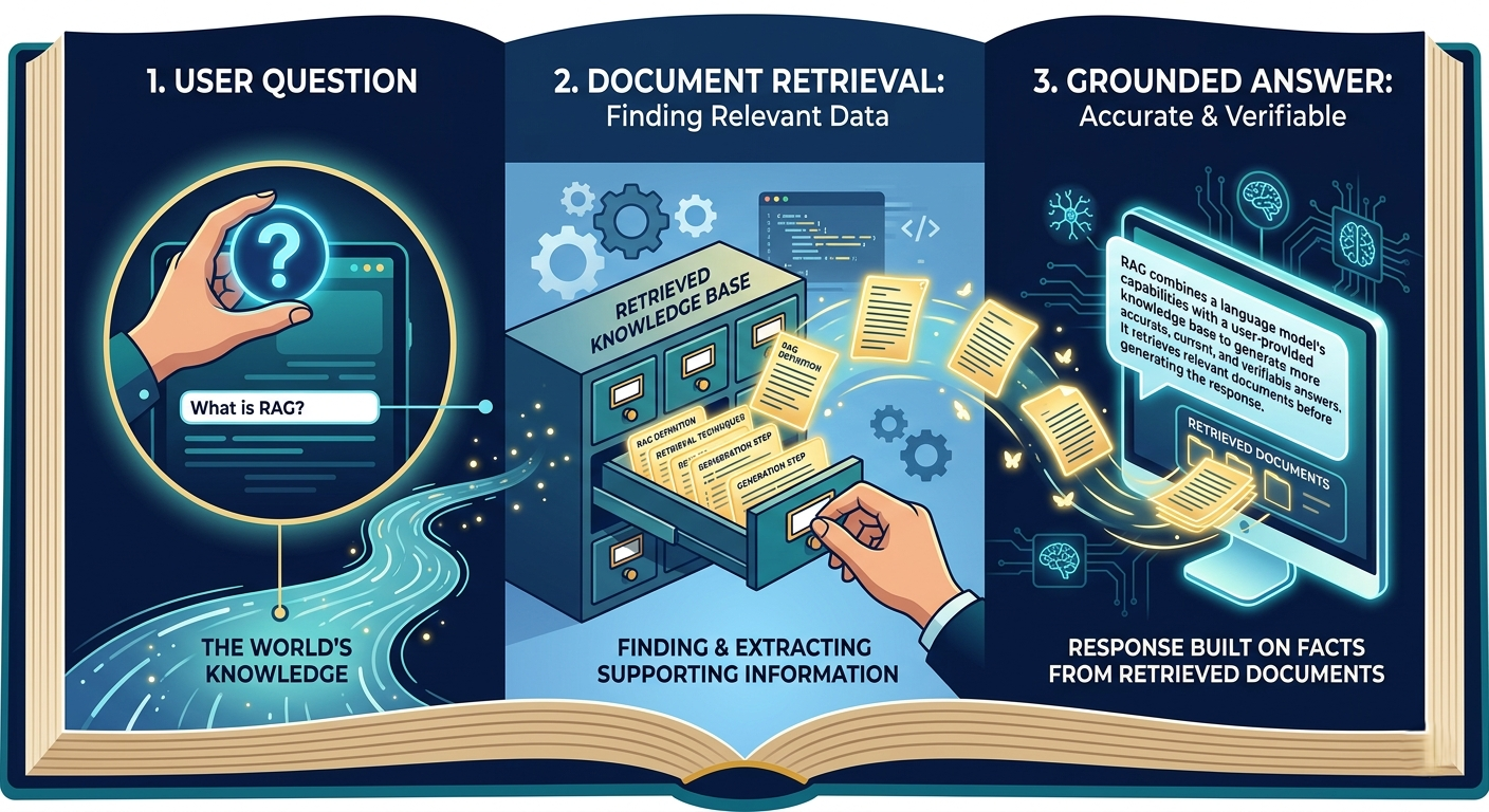
RAG stands for Retrieval-Augmented Generation, and each word in that name describes a distinct phase of the process. Retrieval is the search step: given a user's question, find the most relevant pieces of information from your knowledge base. Augmentation is the injection step: take those retrieved pieces and add them to the prompt you send to the LLM, so the model has access to the relevant facts. Generation is the answer step: the LLM generates a response grounded in the provided context rather than relying solely on its training weights.

The elegant part of RAG is what it doesn't change. Your LLM is still doing what it's best at — reasoning, synthesizing, and producing coherent, well-structured language. You're not fine-tuning the model or retraining it every time your documents update. You're just augmenting its input with the right information at runtime. Update your HR policy document? The next question about parental leave will retrieve the new version automatically. No retraining. No redeployment. Just update the vector database.

Real-World Analogy

Think of RAG like taking an open-book exam. The LLM without RAG is like a student who must answer every question from memory — brilliant for well-covered topics, dangerously wrong for specifics they never studied. RAG gives the student a library card. Before answering, they quickly search the library for the most relevant chapters, read those specific pages, and then write their answer informed by the actual source material. Same intelligence, infinitely better accuracy on domain-specific questions.

# The RAG flow in pseudocode — simple but complete
def rag_query(question: str, knowledge_base, llm) -> str:

 # Step 1: RETRIEVAL — find relevant context
 relevant_chunks = knowledge_base.similarity_search(question, k=4)

 # Step 2: AUGMENTATION — build the augmented prompt
 context = "\n\n".join([chunk.page_content for chunk in relevant_chunks])
 prompt = f"""Answer the question using ONLY the context below.
If the answer isn't in the context, say "I don't have that information."

Context:
{context}

Question: {question}"""

 # Step 3: GENERATION — grounded response
 return llm.invoke(prompt).content

⚡ Pro Tips — RAG Fundamentals

• Always instruct the LLM explicitly to stay within the provided context. Without this instruction, models will blend retrieved facts with their training knowledge, defeating the purpose of RAG.
• Return source citations alongside the answer. Telling users which document and chunk the answer came from is critical for trust and auditability in enterprise applications.
• RAG and fine-tuning solve different problems. RAG grounds responses in current, dynamic data. Fine-tuning adjusts model behavior, tone, and domain-specific reasoning patterns. Use both for production systems that need both.

Search Methods

Keyword vs Semantic Search — Why Word Matching Isn't Enough

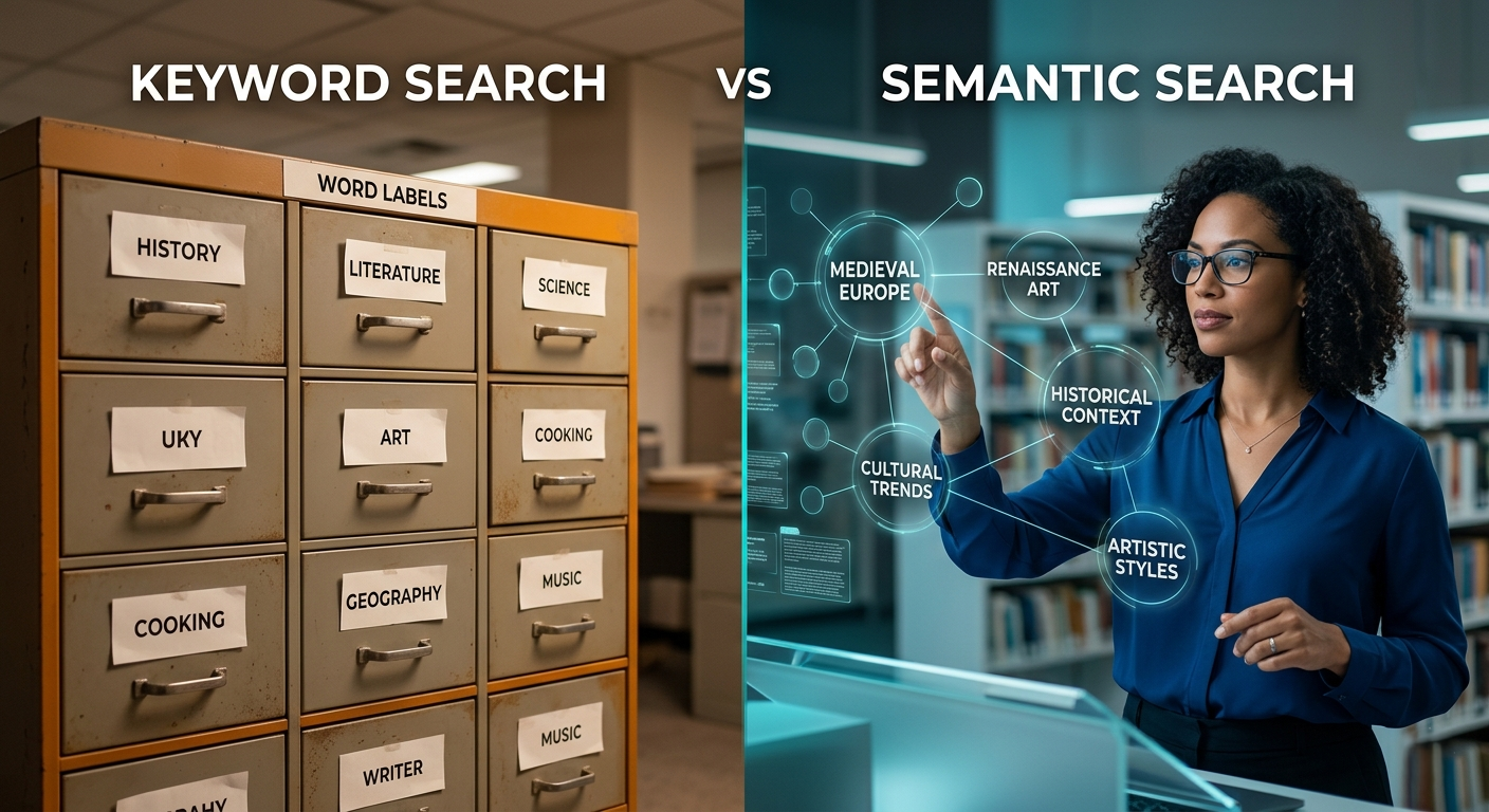
The first major decision in any RAG system is how to find relevant documents. The naive approach — and often the first thing people try — is keyword search. Algorithms like TF-IDF (Term Frequency-Inverse Document Frequency) and BM25 (the engine behind most traditional search engines, including Elasticsearch) work by counting word occurrences. A query for "remote work policy" will match documents containing those exact words, weighted by how frequently they appear and how rare they are across the corpus. For many tasks, this works reasonably well. For understanding meaning, it fundamentally breaks.

Here's the concrete failure mode: a user asks "Can I work from home?" Your HR policy document contains the phrase "remote work is permitted for all employees." Keyword search finds zero overlap between "work from home" and "remote work." The query and the answer literally share no meaningful keywords. A user asking "Is the API down?" won't find a document titled "Service disruption notice." TF-IDF and BM25 don't understand that "work from home," "remote work," and "telecommuting" are semantically equivalent — they only see character sequences. Semantic search, powered by embeddings, solves this by operating in meaning-space rather than word-space.

Real-World Analogy

Keyword search is like searching a filing cabinet by looking for folders with matching labels. You ask for "car repair" and miss everything filed under "automobile maintenance" and "vehicle servicing." Semantic search is like having a librarian who understands what you mean and retrieves everything thematically relevant — regardless of the exact words on the folder label. Same cabinet. Completely different retrieval quality.

# Keyword search with BM25 (rank_bm25 library)
from rank_bm25 import BM25Okapi

corpus = [
 "Remote work is permitted for all employees.",
 "Our office is open Monday to Friday.",
 "Telecommuting benefits include reduced commute times."
]
tokenized = [doc.split() for doc in corpus]
bm25 = BM25Okapi(tokenized)

query = "Can I work from home?"
scores = bm25.get_scores(query.split())
print(scores)
# Output: [0.0, 0.0, 0.0] — no keyword matches found!
# Semantic search would score doc[0] and doc[2] highly.

⚡ Pro Tips — Search Strategy

• Don't abandon keyword search entirely. Use hybrid search — a weighted combination of BM25 (for exact term matching) and semantic search (for meaning). Hybrid search significantly outperforms either alone, especially for queries that mix specific terms with conceptual questions.
• BM25 still wins for exact match requirements: product codes, error codes, regulatory identifiers, and any query where the precise term is critical. Build a router that selects the search strategy based on query type.
• Here's the thing most tutorials miss: semantic search degrades for very short queries (1–2 words) because there isn't enough context to produce a meaningful embedding. Hybrid search is especially valuable for short queries where BM25 provides crucial signal.

Embeddings

Embeddings — Converting Meaning Into Math

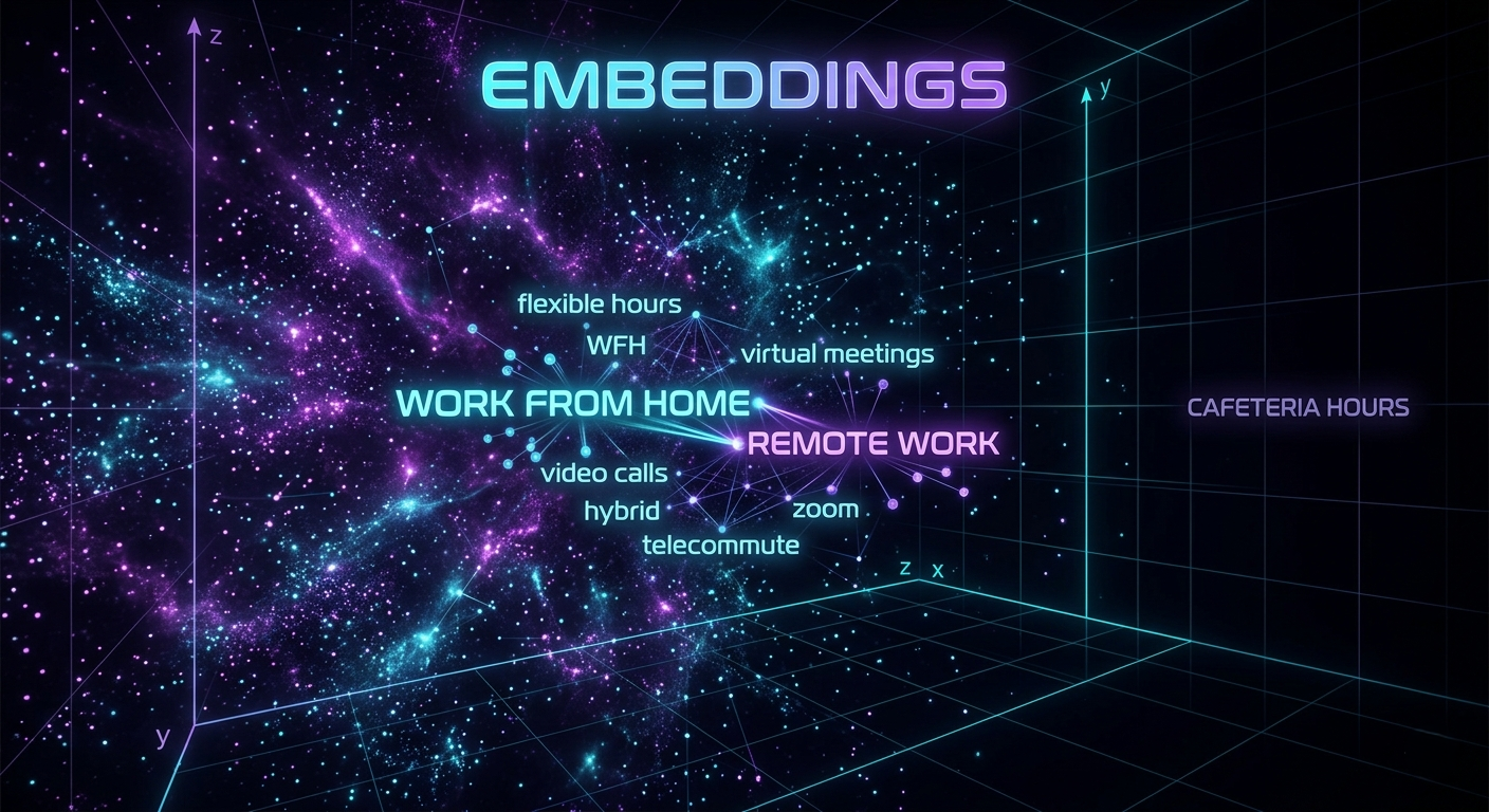
An embedding is a dense numerical vector — typically 384 to 1536 numbers — that encodes the semantic meaning of a piece of text. Embedding models (like OpenAI's text-embedding-3-small or Hugging Face's sentence-transformers/all-MiniLM-L6-v2) are trained on massive text corpora to position semantically similar texts close together in this high-dimensional vector space. "The meeting was cancelled" and "The appointment was called off" will produce vectors that are nearly identical. "The stock market crashed" will be very far away.

The distance between two vectors directly measures semantic similarity. Cosine similarity is the standard metric: it measures the angle between two vectors, yielding a score from 0 (orthogonal — completely unrelated) to 1 (parallel — identical meaning). This mathematical representation of meaning is what allows you to find "Can I work from home?" — even though the relevant document says "remote work permitted" — because both phrases occupy nearby positions in embedding space. The model was trained to understand that these phrases convey the same intent.

Choosing the right embedding model matters more than most people realize. Larger models (1536 dimensions, like OpenAI's ada-002) capture more nuanced semantic relationships but cost more to compute and store. Smaller models (384 dimensions, like MiniLM) are fast, free to run locally, and sufficient for most enterprise RAG tasks. The critical constraint: whatever model you use to embed your documents, you must use the same model to embed queries at retrieval time. Different models produce incompatible vector spaces — a query embedded with model A cannot be meaningfully compared to documents embedded with model B.

from sentence_transformers import SentenceTransformer
import numpy as np

model = SentenceTransformer("all-MiniLM-L6-v2") # 384 dims, free, fast

sentences = [
 "Can I work from home?",
 "Remote work is permitted for all employees.",
 "The office cafeteria serves lunch until 2pm."
]
embeddings = model.encode(sentences)
print(embeddings.shape) # (3, 384)

# Cosine similarity — 1.0 = identical meaning, 0.0 = unrelated
def cosine_sim(a, b):
 return np.dot(a, b) / (np.linalg.norm(a) * np.linalg.norm(b))

print(cosine_sim(embeddings[0], embeddings[1])) # ~0.72 (similar!)
print(cosine_sim(embeddings[0], embeddings[2])) # ~0.12 (unrelated)

⚡ Pro Tips — Embeddings

• Don't embed your entire document as one vector. A 50-page PDF produces a single embedding that averages across all topics in the document — it will be mediocre at representing any specific section. Chunk first, then embed (covered in the chunking section).
• For multilingual applications, use multilingual embedding models like paraphrase-multilingual-MiniLM-L12-v2. These can embed text from 50+ languages into the same vector space, enabling cross-language retrieval.
• Embedding costs are one-time per document. You pay to embed when you ingest a document, then retrieval is just a vector similarity search — cheap and fast. Don't re-embed documents unless the embedding model changes or the document content changes.

Vector Databases

ChromaDB — Storing and Searching Millions of Vectors

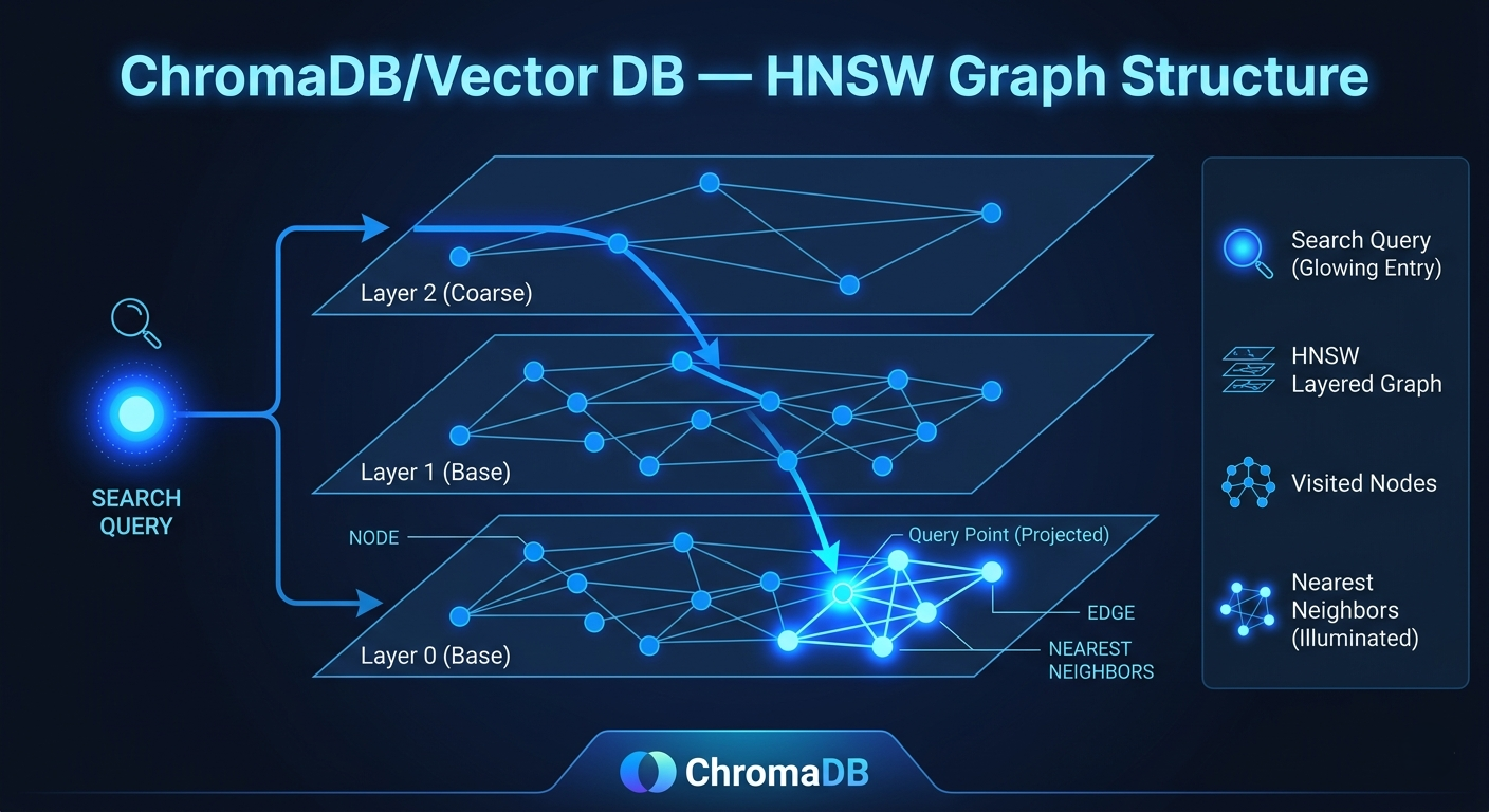
Once you have embeddings, you need somewhere efficient to store them and — critically — search through them quickly. A regular database can store vectors as arrays, but performing cosine similarity comparisons against millions of vectors one-by-one would take minutes. Vector databases solve this with approximate nearest neighbor (ANN) algorithms like HNSW (Hierarchical Navigable Small World graphs) that can find the top-K most similar vectors in milliseconds, even across millions of documents. They're the index that makes semantic search practical at scale.

ChromaDB is the go-to choice for development and small-to-medium production workloads. It runs locally with zero configuration, persists to disk, handles filtering and metadata alongside vectors, and integrates natively with LangChain. For larger scale, Pinecone (managed, serverless), Weaviate (open source, hybrid search built-in), and Qdrant (Rust-based, extremely fast) are production favorites. The API patterns are nearly identical — so building with ChromaDB locally means very little rework when migrating to a production vector store.

import chromadb
from sentence_transformers import SentenceTransformer

# Initialize persistent ChromaDB
client = chromadb.PersistentClient(path="./chroma_db")
collection = client.get_or_create_collection(
 name="company_docs",
 metadata={"hnsw:space": "cosine"} # cosine similarity metric
)

model = SentenceTransformer("all-MiniLM-L6-v2")

# Ingest documents
docs = [
 "Remote work is permitted for all full-time employees.",
 "Parental leave is 12 weeks fully paid.",
 "Annual performance reviews occur in December."
]
embeddings = model.encode(docs).tolist()

collection.add(
 documents=docs,
 embeddings=embeddings,
 ids=[f"doc_{i}" for i in range(len(docs))],
 metadatas=[{"source": "hr_policy_v2.pdf"}] * len(docs)
)

# Query
query = "Can I work from home?"
q_emb = model.encode([query]).tolist()
results = collection.query(query_embeddings=q_emb, n_results=2)
print(results["documents"]) # ["Remote work is permitted...", ...]

⚡ Pro Tips — Vector Databases

• Always store metadata alongside your vectors: source file, page number, document date, author, and section title. At retrieval time, you can filter by metadata before the vector search, dramatically improving precision for targeted queries.
• ANN algorithms trade exactness for speed. HNSW is approximate — it might miss the single closest vector 1–5% of the time. For most RAG applications, this is completely acceptable. For high-stakes applications, increase ef_search (the search expansion factor) to get closer to exact results at the cost of some latency.
• Don't use one giant collection for everything. Partition by domain (HR docs, engineering docs, customer support) and route queries to the right collection based on context. Cross-domain retrieval introduces noise that degrades answer quality.

Document Chunking

Document Chunking — The Detail That Breaks Most RAG Systems

This is the section where most RAG tutorials let you down. They tell you to "split your documents into chunks" and move on. But chunk strategy is arguably the most impactful variable in your entire RAG pipeline — more important than your choice of embedding model, more important than your vector database. Get chunking wrong and your retrieval will be mediocre regardless of everything else.

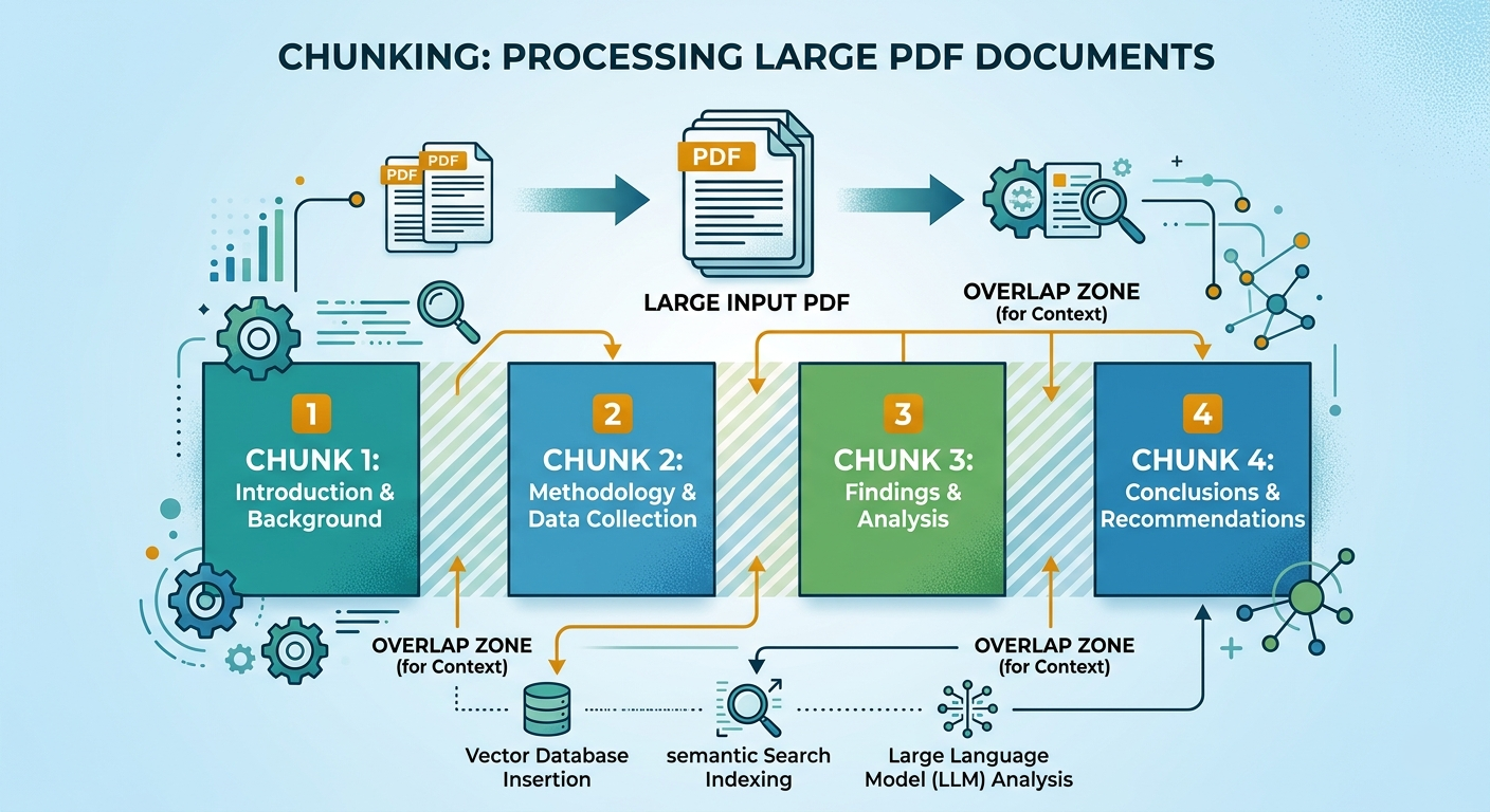
The fundamental tradeoff: large chunks contain more context but produce noisier, less precise embeddings. A 2,000-word chunk embedding tries to represent the meaning of a lot of content — it becomes a blurry average. A 200-word chunk produces a sharp, focused embedding but might miss the surrounding context needed to answer certain questions. The right chunk size depends on your document type, your query patterns, and your LLM's context window. For most enterprise document RAG (PDFs, policies, manuals), chunk sizes between 512 and 1024 tokens with a 10–20% overlap work well as a starting baseline.

Chunk overlap — repeating the last N tokens of one chunk at the start of the next — solves the boundary problem: if a key sentence falls exactly at a chunk boundary, overlap ensures it's fully represented in at least one chunk. Without overlap, answers that require a complete sentence spanning a boundary will be systematically missed. Beyond fixed-size splitting, more sophisticated strategies include recursive character splitting (respects paragraph and sentence boundaries), semantic chunking (dynamically groups sentences with high embedding similarity), and document-structure-aware chunking (splits on headings, sections, and list structures).

from langchain_text_splitters import RecursiveCharacterTextSplitter

# Recursive splitter — tries to split on paragraphs, then sentences
splitter = RecursiveCharacterTextSplitter(
 chunk_size=800, # ~200 words, good general starting point
 chunk_overlap=100, # 12.5% overlap — prevents boundary gaps
 length_function=len,
 separators=["\n\n", "\n", ". ", " ", ""] # priority order
)

with open("hr_policy.txt") as f:
 document = f.read()

chunks = splitter.create_documents([document])
print(f"Document split into {len(chunks)} chunks")
print(f"Sample chunk: {chunks[0].page_content[:200]}")

# For PDFs with page awareness:
from langchain_community.document_loaders import PyPDFLoader
loader = PyPDFLoader("hr_policy.pdf")
pages = loader.load_and_split(text_splitter=splitter)
# Each chunk retains page metadata for citation

⚡ Pro Tips / Common Mistakes — Chunking

• Never chunk across section boundaries. An HR policy document has sections like "Vacation Policy," "Remote Work," and "Benefits." Split at section headers first, then apply character splitting within sections. Mixing content from different sections into one chunk confuses retrieval.
• Measure chunk quality empirically. Generate 20 representative questions, retrieve chunks, and manually evaluate whether the right chunks come back. Chunk size "feels" right intuitively but only data can tell you what actually works for your specific corpus.
• For tables and structured data inside documents, extract and format them separately before chunking. A PDF table chunked naively looks like garbled text to an embedding model. Extract table rows as structured strings ("Column A: value, Column B: value") then embed those.
• Token count ≠ character count. If your LLM context window is measured in tokens, use a tokenizer-aware splitter to ensure chunks fit. tiktoken for OpenAI models gives you exact token counts.

The RAG Pipeline

Building the Complete RAG Pipeline — Putting It All Together

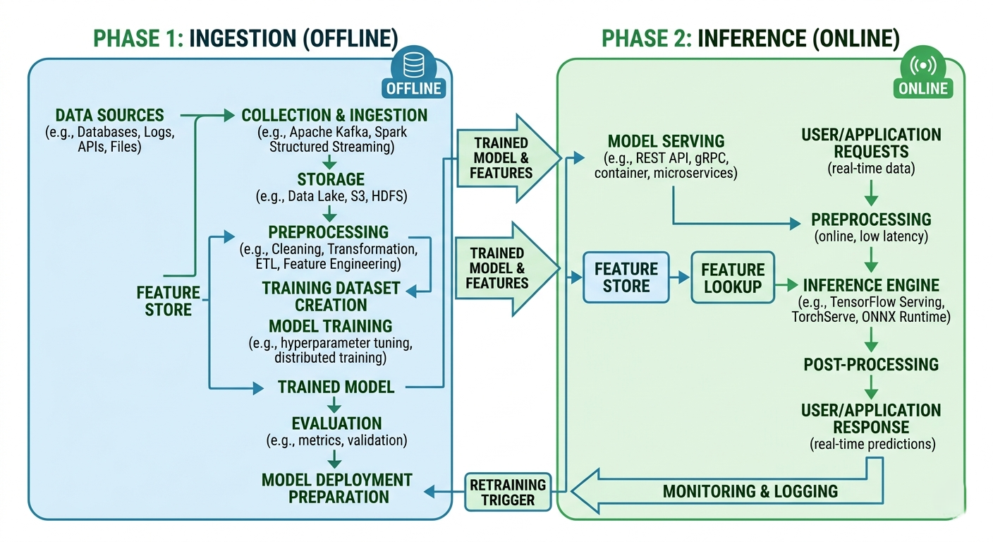
With all the components understood individually, the full RAG pipeline becomes straightforward to assemble. There are two distinct phases: ingestion (the offline phase that runs once per document set) and inference (the online phase that runs for every user query). Getting this distinction right in your architecture is crucial — ingestion can be slow and expensive, inference needs to be fast.

The ingestion phase: load documents → split into chunks → generate embeddings for each chunk → store chunks and embeddings in your vector database with metadata. This can take minutes to hours depending on corpus size, but it only runs when documents change. The inference phase: receive query → embed the query (milliseconds) → vector similarity search to retrieve top-K chunks (milliseconds) → construct augmented prompt with retrieved context → send to LLM → return answer with sources. End-to-end inference latency for a well-built RAG system should be under 3 seconds for most queries.

from langchain_community.vectorstores import Chroma
from langchain_openai import OpenAIEmbeddings, ChatOpenAI
from langchain_text_splitters import RecursiveCharacterTextSplitter
from langchain_community.document_loaders import PyPDFLoader
from langchain.chains import RetrievalQA

# ── INGESTION PHASE (runs once per document update) ──────────
loader = PyPDFLoader("company_handbook.pdf")
docs = loader.load()

splitter = RecursiveCharacterTextSplitter(chunk_size=800, chunk_overlap=100)
chunks = splitter.split_documents(docs)

embeddings = OpenAIEmbeddings(model="text-embedding-3-small")
vectorstore = Chroma.from_documents(
 documents=chunks,
 embedding=embeddings,
 persist_directory="./chroma_store"
)
print(f"Ingested {len(chunks)} chunks")

# ── INFERENCE PHASE (runs for every user query) ──────────────
vectorstore = Chroma(
 persist_directory="./chroma_store",
 embedding_function=embeddings
)
retriever = vectorstore.as_retriever(
 search_type="similarity",
 search_kwargs={"k": 4}
)

qa_chain = RetrievalQA.from_chain_type(
 llm=ChatOpenAI(model="gpt-4o", temperature=0),
 retriever=retriever,
 return_source_documents=True
)

result = qa_chain.invoke({"query": "What is the parental leave policy?"})
print(result["result"])
print("\nSources:")
for doc in result["source_documents"]:
 print(f" - {doc.metadata.get('source')}, page {doc.metadata.get('page')}")

⚡ Pro Tips — Pipeline Construction

• Set LLM temperature to 0 for RAG pipelines. You want the model to extract and present facts from the context, not creatively embellish them. Temperature 0 gives you the most faithful, deterministic responses.
• Always implement a fallback for "I don't know." If retrieved chunks have low similarity scores (below your threshold), don't force the LLM to answer — return a structured "no information found" response rather than a hallucinated answer dressed up as retrieval-backed.
• Separate ingestion from inference in your infrastructure. Ingestion runs asynchronously on document updates. Inference is your hot path. They have completely different performance and cost profiles and should be scaled independently.

Production

Production Deployment — From Prototype to Reliable System

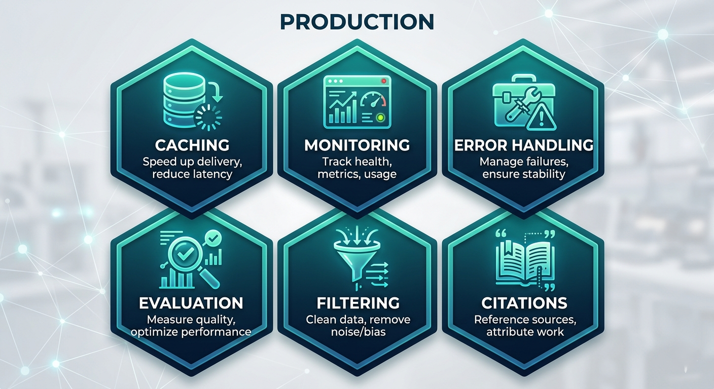
A RAG prototype that works on 50 test queries is very different from a production system handling 10,000 queries per day with SLA guarantees. The gap between them is filled by four engineering concerns that are rarely covered in tutorials: caching, monitoring, error handling, and evaluation. Skipping any one of these in production is how "the AI is broken" incidents happen at 2 AM on a Saturday.

Caching is your biggest lever for both latency and cost. Identical or near-identical queries (common in enterprise chatbots where dozens of employees ask similar HR questions) should hit a semantic cache rather than re-running the full embedding + retrieval + generation pipeline. GPTCache and Redis with vector search are popular choices. Monitoring means tracking retrieval metrics (chunk similarity scores, whether the answer was grounded in context), LLM response quality (via automated evaluators or human review sampling), and system health (latency percentiles, error rates). Without monitoring, RAG quality silently degrades as documents age and query patterns change. Error handling means gracefully managing embedding API failures, vector store connection issues, and LLM rate limits — with circuit breakers, retries with backoff, and meaningful error messages to users rather than opaque failures.

import time
from functools import lru_cache
import logging

# Production RAG with caching, retry, and monitoring
logger = logging.getLogger("rag_pipeline")

class ProductionRAG:
 def __init__(self, vectorstore, llm, cache_ttl=3600):
 self.vectorstore = vectorstore
 self.llm = llm
 self.cache = {}
 self.cache_ttl = cache_ttl

 def query(self, question: str, min_similarity: float = 0.6) -> dict:
 # Check cache first
 cache_key = question.lower().strip()
 if cache_key in self.cache:
 logger.info("Cache hit")
 return self.cache[cache_key]

 start = time.time()
 try:
 # Retrieve with similarity scores
 results = self.vectorstore.similarity_search_with_score(question, k=4)
 high_quality = [(doc, score) for doc, score in results if score >= min_similarity]

 if not high_quality:
 logger.warning(f"Low confidence retrieval for: {question}")
 return {"answer": "I couldn't find relevant information.", "sources": []}

 context = "\n\n".join([doc.page_content for doc, _ in high_quality])
 answer = self.llm.invoke(f"Answer using context only:\n{context}\n\nQ: {question}").content
 sources = [doc.metadata.get("source", "unknown") for doc, _ in high_quality]

 response = {"answer": answer, "sources": sources,
 "latency_ms": (int((time.time() - start) * 1000))}

 self.cache[cache_key] = response # cache result
 logger.info(f"Query answered in {response['latency_ms']}ms")
 return response

 except Exception as e:
 logger.error(f"RAG query failed: {e}")
 raise

⚡ Pro Tips — Production RAG

• Implement RAG evaluation with frameworks like RAGAS or TruLens. These automatically score your system on faithfulness (is the answer grounded in context?), answer relevancy (does it address the question?), and context precision (are retrieved chunks relevant?). Run evaluations on a golden test set before every deployment.
• Version your vector collections. When you update documents or change chunk strategy, create a new collection rather than updating in place. Keep the old collection running until the new one is validated. Blue-green deployment for vector databases.
• Set similarity score thresholds tightly in the beginning, then loosen as you gather data. Starting with a high threshold (0.75+) means you'll return "I don't know" often, but the answers you do return will be trustworthy. Adjust down once you've measured false negative rates.

Synthesis

How It All Connects — The Full RAG Mental Model

Let's trace the complete journey of a user's question through a production RAG system and see how every component we've covered plays its role. An HR manager types: "What are the rules around taking parental leave while on a performance improvement plan?" That question arrives at your API. The query is immediately embedded using the same model that embedded your documents — producing a 384-dimensional vector that encodes the semantic meaning of the question. This takes about 20 milliseconds.

That query vector is then sent to ChromaDB's HNSW index, which searches across 50,000 stored chunk embeddings and returns the top 4 most similar ones in under 50 milliseconds — even though an exhaustive search would take seconds. Those 4 chunks were created during ingestion: your HR policy PDF was loaded, recursively split into 800-character chunks with 100-character overlaps, each chunk embedded and stored with metadata (page number, section, document version). The retrieved chunks cover parental leave duration, PIP procedures, and a relevant clause about leave eligibility.

These chunks are inserted into a carefully constructed prompt that instructs the LLM to answer only from the provided context. The LLM generates a precise, cited response in about 2 seconds. The full round-trip: under 3 seconds. The answer: accurate, grounded in your actual policy, and returned with source citations so the manager can verify. That's the power of a well-built RAG system — and every component from chunking strategy to similarity threshold contributed to making that answer trustworthy.

Getting Started

Getting Started — Build Your First RAG System in 30 Minutes

# Step 1: Install dependencies
pip install langchain langchain-openai langchain-community \
 chromadb sentence-transformers rank-bm25 \
 pypdf tiktoken

# Step 2: Set API key
export OPENAI_API_KEY="your-key-here"

# Step 3: Create and populate your knowledge base
from langchain_community.document_loaders import PyPDFLoader, TextLoader
from langchain_text_splitters import RecursiveCharacterTextSplitter
from langchain_community.vectorstores import Chroma
from langchain_openai import OpenAIEmbeddings, ChatOpenAI
from langchain.chains import RetrievalQA

# Load your documents (PDF or text)
loader = TextLoader("your_document.txt") # or PyPDFLoader("doc.pdf")
docs = loader.load()

# Chunk them
splitter = RecursiveCharacterTextSplitter(chunk_size=800, chunk_overlap=100)
chunks = splitter.split_documents(docs)
print(f"✓ {len(chunks)} chunks created")

# Embed and store
embed_model = OpenAIEmbeddings(model="text-embedding-3-small")
vectorstore = Chroma.from_documents(chunks, embed_model, persist_directory="./my_rag_db")
print(f"✓ Vector store populated")

# Step 4: Build and run your RAG chain
qa = RetrievalQA.from_chain_type(
 llm=ChatOpenAI(model="gpt-4o", temperature=0),
 retriever=vectorstore.as_retriever(search_kwargs={"k": 4}),
 return_source_documents=True
)

# Step 5: Ask questions
questions = [
 "What is the remote work policy?",
 "How long is parental leave?",
 "When are performance reviews conducted?"
]
for q in questions:
 result = qa.invoke({"query": q})
 print(f"\nQ: {q}")
 print(f"A: {result['result']}")
 print(f"Sources: {set(d.metadata.get('source','') for d in result['source_documents'])}")

FAQ

Frequently Asked Questions

What is RAG in AI and why is it needed? RAG (Retrieval-Augmented Generation) is a technique that grounds LLM responses in external, up-to-date documents rather than relying solely on training data. It's needed because LLMs have a knowledge cutoff date, don't have access to private/proprietary data, and hallucinate when asked about specifics outside their training. RAG solves all three problems without requiring model retraining. What's the difference between RAG and fine-tuning? Fine-tuning adjusts the model's weights to change its behavior, reasoning patterns, and domain-specific language — it "teaches" the model. RAG provides the model with relevant information at query time — it "shows" the model. Fine-tuning is better for style, tone, and behavior changes. RAG is better for dynamic, current, or proprietary knowledge. For production systems, both are often combined. What is the best chunk size for RAG? There's no universal best chunk size — it depends on your document type, query patterns, and LLM context window. A good starting point: 512–1024 characters with 10–20% overlap for prose documents like policies and manuals. For technical documentation or code, smaller chunks (256–512) with higher overlap work better. Always empirically evaluate by running representative queries and checking whether correct chunks are retrieved. Which vector database should I use for RAG? For development and small production workloads: ChromaDB (local, no cost, easy setup). For production scale: Pinecone (fully managed, serverless), Weaviate (open source, hybrid search built-in), Qdrant (extremely fast, Rust-based), or pgvector (if you're already on PostgreSQL). The API patterns are nearly identical, so start with ChromaDB and migrate when you hit scale limits. How do I prevent hallucinations in my RAG system? Four measures: (1) Set temperature to 0 on the LLM to minimize creative generation. (2) Explicitly instruct the model to answer only from provided context and say "I don't know" if the answer isn't there. (3) Set a minimum similarity threshold on retrieved chunks — don't send low-confidence chunks to the LLM. (4) Use faithfulness evaluation (RAGAS) to automatically score whether answers are grounded in retrieved context. What embedding model should I use for RAG? For general-purpose enterprise RAG: text-embedding-3-small (OpenAI, 1536 dims, excellent quality) or all-MiniLM-L6-v2 (Hugging Face, 384 dims, free, runs locally, very good quality). For multilingual: paraphrase-multilingual-MiniLM-L12-v2. Critical rule: use the same embedding model for both ingestion and query time — mixed models produce incompatible vector spaces. How do I handle documents that update frequently? Implement incremental ingestion: track document versions/timestamps, and re-embed only changed or new documents rather than rebuilding the entire vector store. Use document IDs in your vector store so you can delete-and-replace specific document chunks. For real-time documents (live databases, news feeds), consider streaming ingestion pipelines that process updates as they arrive. Can RAG work without OpenAI? Completely. Use local embedding models (sentence-transformers) with ChromaDB or Qdrant for the retrieval layer. Use local LLMs (Ollama with Llama 3, Mistral, or Phi-3) for generation. Anthropic Claude, Google Gemini, and Cohere all work as drop-in LLM replacements. A fully local, zero-API-cost RAG system is practical for most enterprise use cases with reasonable hardware.

🔬 RAG Interactive Lab

Visualize embeddings, compare keyword vs semantic search, experiment with chunking, and run a complete RAG pipeline — all in your browser.

Embedding Similarity Visualizer

See how semantically similar texts produce similar vector patterns. Colors represent embedding dimensions — similar texts have similar color patterns.

Vector Space Visualization Sentence A Can I work from home? EMBEDDING VECTOR (first 32 dims) Sentence B Remote work is permitted for all employees. EMBEDDING VECTOR (first 32 dims) Cosine Similarity Scores A vs B (above) — "office cafeteria hours" — "telecommuting benefits" —

💡 Try editing Sentence A or B and re-running to see how similarity changes. Try making them very similar vs very different.

Keyword vs Semantic Search — Live Comparison

Type a query. See which documents each method retrieves — and why semantic search wins for meaning-based queries.

Knowledge Base: HR Policy Docs 🔤 Keyword Search (BM25/TF-IDF) Run a search to see results 🧠 Semantic Search (Embeddings) Run a search to see results Try these queries:

Chunking Visualizer — Size & Overlap

Drag the slider to change chunk size. See how the document splits — and where overlap prevents information gaps at boundaries.

Document Chunker — chunks Chunk size: 120 chars Loading…

Complete RAG Pipeline Simulation

Ask a question about the simulated HR policy knowledge base. Watch each pipeline step execute and see how the answer is grounded in retrieved chunks.

Pipeline Execution Idle 🔢 Embed Query Convert question to 384-dim vector using sentence-transformers waiting 🔍 Vector Retrieval HNSW search across 50k chunks → top-4 by cosine similarity waiting 📋 Augment Prompt Inject retrieved chunks into LLM prompt with context instructions waiting 🤖 Generate Answer LLM produces grounded response with citations waiting Generated Answer (Grounded in Retrieved Context) Execution Log

Production Architecture Checklist

Click each card to mark it as implemented. A production-ready RAG system needs all six.

Production Readiness 0 / 6 ⚡ Semantic Caching Cache similar queries using GPTCache or Redis with vector search. Reduces cost 40–70% in enterprise chatbots. 📊 RAG Evaluation RAGAS scores: faithfulness, answer relevancy, context precision. Run on golden test set before each deployment. 🔄 Error Handling Circuit breakers, retries with backoff, similarity threshold gates, graceful "I don't know" fallbacks. 📡 Monitoring Track latency percentiles, similarity score distributions, retrieval quality, and LLM token usage per query. 🏷️ Metadata Filtering Pre-filter by doc type, date, department before vector search. Improves precision 2–3× for targeted queries. 📋 Source Citations Return document name, page number, and section for every answer. Required for enterprise trust and auditability.

Knowledge Check — Test Your RAG Understanding

8 questions covering the full RAG pipeline.