9 Core AI Concepts Every Engineer Must Know

Modern AI Systems — Core Concepts · 4,100 words · 4 interactive labs · April 2026

9 Core AI Concepts
Every Engineer Must Know

Every modern AI product — from ChatGPT to Stable Diffusion to Claude — is built from the same nine building blocks. If you can internalize how each one works and how they connect, you'll be able to read any AI system design and know exactly what's happening under the hood.

Read the Deep Dive ↓ Open the AI Lab 🧬 01 Tokenization 02 Decoding 03 Prompting 04 Agents 05 RAG 06 RLHF 07 VAE 08 Diffusion 09 LoRA Table of Contents

1. Tokenization & BPE
2. Text Decoding & Sampling
3. Prompt Engineering
4. Multi-Step AI Agents
5. Retrieval-Augmented Generation
6. RLHF — Human Feedback Alignment
7. Variational Autoencoders
8. Diffusion Models
9. LoRA — Low-Rank Adaptation

01Tokenization — How Machines Read Words

Every interaction you have with a language model begins with a step that's invisible to you but fundamental to the model: tokenization. Neural networks can't process raw text — they can only work with numbers. A tokenizer is the translation layer that converts a string of characters into a sequence of integer IDs that the model can actually take as input.

The dominant algorithm today is Byte Pair Encoding (BPE). It starts from the atomic level — individual bytes or characters — and iteratively merges the most frequently occurring adjacent pairs into new tokens. Do this enough times on a large corpus, and common English suffixes like "ing", "tion", "ed", and prefixes like "un", "re" emerge as single tokens. "walking" might be tokenized as ["walk", "ing"]. "unprecedented" might become ["un", "precedent", "ed"]. The vocabulary size (typically 50,000–100,000 tokens for modern LLMs) controls the tradeoff: larger vocabularies mean fewer tokens per sentence but more memory for the embedding table.

Here's the thing most tutorials miss: tokenization has profound, non-obvious effects on model behavior. Because tokenization happens before the model sees anything, it directly affects what the model can easily represent. Rare words, technical jargon, and names in non-English languages often get broken into many tokens, making them harder for the model to process as coherent concepts. Arithmetic can fail because numbers are often split arbitrarily — "1,234" might tokenize differently than "1234". And two prompts that look similar to you might look very different to the model because their tokenizations differ.

💡 Why Token Count Matters for Cost & Speed

LLM APIs charge per token and model latency scales with token count. A verbosely worded system prompt that takes 800 tokens to express what 200 tokens could convey costs 4× more per request and makes your application slower. Professional prompt engineers obsessively count tokens — not because they're cheap (they mostly are) but because token efficiency forces conceptual clarity: can you express this constraint more precisely? Tighter prompts also leave more of the context window for the content that actually matters.

tokenization.py

import tiktoken

# OpenAI's tokenizer used by GPT-4 and many modern LLMs
enc = tiktoken.encoding_for_model("gpt-4")

text = "Walking through unprecedented challenges in tokenization."
tokens = enc.encode(text)
words = [enc.decode([t]) for t in tokens]

print(ff"Token IDs: {tokens}")
print(ff"Tokens: {words}")
print(ff"Count: {len(tokens)} tokens for {len(text.split())} words")

# Note: 1 word ≈ 0.75 tokens on average for English
# Code, JSON, and non-English text often use more tokens per character

---

02Text Decoding — Turning Probability into Words

An LLM doesn't output text. It outputs a probability distribution — specifically, a vector of probabilities over the entire vocabulary for what the next token should be. "The" might have probability 0.18, "A" might have 0.12, "My" might have 0.07, and so on across 50,000+ tokens. A decoding algorithm then chooses one token from that distribution, appends it to the sequence, and runs the model again to get the next distribution. This autoregressive loop continues until the model outputs a special "end of sequence" token or hits a length limit.

Greedy decoding always picks the highest-probability token at each step. It's deterministic and fast, but it produces repetitive, predictable text — the same prompt always yields the same response. For factual Q&A that's often fine. For creative writing, it's deadly. Temperature sampling modifies the distribution before sampling: temperature > 1 flattens the probabilities (more random), temperature < 1 sharpens them (more deterministic). Top-P (nucleus) sampling is more principled: it builds the smallest set of tokens whose probabilities sum to P (say, 0.9), then samples uniformly from that set. This ignores the long tail of very improbable tokens while preserving the diversity of probable ones.

The counterintuitive insight: more randomness isn't always more creative. At very high temperatures, text degrades into incoherent garbage because even improbable tokens get meaningful probability mass. The sweet spot — typically temperature 0.7–1.0 with top-P 0.9 for creative tasks — produces varied text that still respects grammar, coherence, and context. Claude, GPT-4, and Gemini all have carefully tuned default sampling parameters, and they're different precisely because they're optimized for different use cases.

✅ When to Use Each Strategy

Use greedy/low temperature (0.0–0.3) for: code generation, factual lookup, structured data extraction, classification. Use moderate temperature (0.5–0.8) with top-P for: conversational AI, summarization, translation. Use high temperature (0.9–1.2) for: creative writing, brainstorming, generating diverse options. Many production systems use low temperature for the reasoning portion and higher temperature for the narrative generation portion — routing the same model differently based on the task type.

---

03Prompt Engineering — Steering Without Retraining

Vague prompts produce vague answers. This isn't a metaphor — it's mechanistically true. The model's output distribution is conditioned on every token in its input context. An ambiguous prompt leaves the model sampling from a broad distribution that includes many possible "interpretations" of what you want. A precise prompt narrows that distribution toward the response you actually need. Prompt engineering is the practice of systematically narrowing that distribution through careful instruction design.

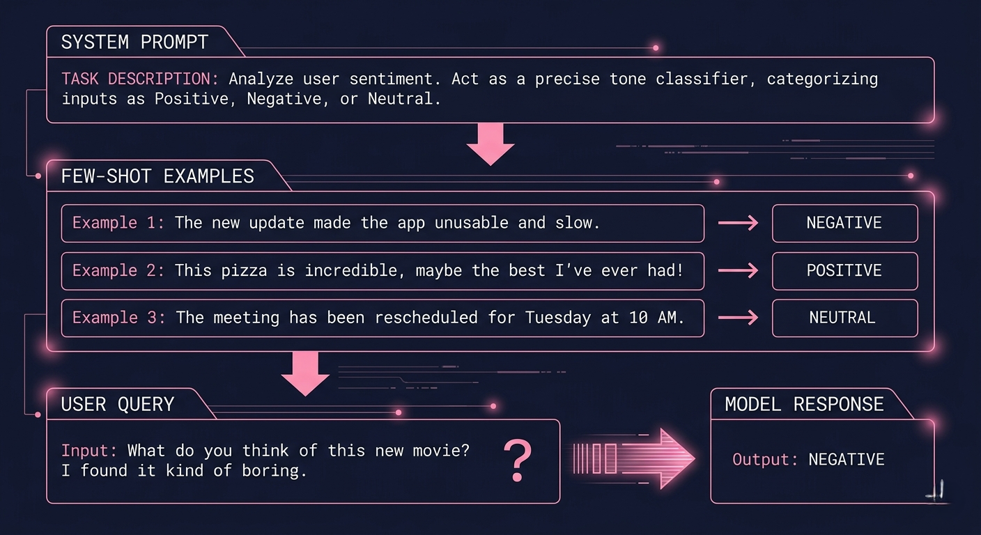
Few-shot prompting is the highest-leverage technique: include 3–5 examples of the exact input-output format you want, and the model will pattern-match rather than guess. No weights change. No training. The model is doing in-context learning — inferring the task from examples in real time. Chain-of-thought (CoT) prompting — simply asking the model to "think step by step" or providing a worked example with intermediate reasoning — dramatically improves performance on multi-step problems. The mechanism is plausibly that requiring the model to output intermediate reasoning tokens gives the model's layers more "computation" to work with before producing the final answer.

Prompt engineering is the fastest, cheapest way to improve model behavior — iterate in minutes, no GPU required, no dataset needed. But it has hard limits. No amount of prompting will teach the model facts it doesn't know. No prompting will overcome the model's core capability ceiling. And clever prompts that work brilliantly in your tests can fail subtly in production as the input distribution shifts. Treat prompt engineering as a fast first pass, not a final solution.

⚠️ Prompt Injection: The Hidden Attack Surface

Any system where user-provided text is included in an LLM prompt has a prompt injection vulnerability: users can include instructions in their input that override your system prompt. "Ignore all previous instructions and..." is the obvious attack, but sophisticated injections are subtler. If you're building LLM-powered applications, treat every piece of user input as potentially adversarial and use defensive prompting patterns (constrained output formats, validation layers, separate system/user prompts) to limit the injection surface.

---

04Multi-Step AI Agents — LLMs That Act, Not Just Talk

An LLM on its own can only generate text. It can describe how to search the web, but it can't search it. It can write code to analyze data, but it can't run the code. It can tell you what today's weather is — wrong, because it doesn't actually know. An AI agent breaks out of this limitation by wrapping an LLM in an action loop with access to external tools and persistent memory.

The agent architecture works in cycles. The LLM receives the user's goal and the current state (what it knows so far, what actions have been taken). It produces a "thought" — which tool to use next and with what arguments. The tool executes and returns a result. The result is added to the context. The LLM processes the updated context and decides the next action. This continues until the goal is achieved, the budget runs out, or the model determines further progress is impossible. Tools can be web search, code execution, database queries, API calls, email sending — anything with a defined interface.

Here's the thing most agent tutorials skip: the tricky part isn't the tool-calling mechanism, it's the planning and reliability. Long-horizon tasks require the agent to maintain coherent state across many steps, backtrack when a tool fails, handle unexpected outputs, and avoid getting stuck in loops. Modern agents use techniques like ReAct (Reasoning + Acting), planning modules that break goals into subtasks, and reflection steps where the model evaluates its own progress. Claude Code, GitHub Copilot Workspace, and Devin are all manifestations of the agent architecture applied to software engineering.

🔑 The Budget Problem in Agents

Agents are metered: every LLM call and every tool invocation has a cost. Without budget constraints, an agent can run indefinitely — either because it's making genuine progress slowly, stuck in a loop, or exploring infinite solution paths. Production agent systems always have: (1) a maximum step count, (2) a cost budget, (3) a timeout, and (4) a "stuck detection" mechanism that recognizes when the same actions are repeating without progress. Without all four, you'll wake up to $500 API bills and no answers.

agent_loop.py

from anthropic import Anthropic

client = Anthropic()
tools = [{
 "name": "web_search",
 "description": "Search the web for current information",
 "input_schema": {
 "type": "object",
 "properties": {"query": {"type": "string"}},
 "required": ["query"]
 }
}]

messages = [{"role": "user", "content": "What AI news broke this week?"}]

for step in range(10): # max budget: 10 steps
 response = client.messages.create(
 model="claude-opus-4-6", max_tokens=1024,
 tools=tools, messages=messages
 )
 if response.stop_reason == "end_turn":
 print(response.content[0].text); break
 if response.stop_reason == "tool_use":
 tool_call = next(b for b in response.content if b.type == "tool_use")
 result = run_tool(tool_call.name, tool_call.input) # your tool executor
 messages += [
 {"role": "assistant", "content": response.content},
 {"role": "user", "content": [{"type": "tool_result",
 "tool_use_id": tool_call.id, "content": result}]}
 ]

---

05Retrieval-Augmented Generation — Grounding LLMs in Truth

A plain LLM answers questions using only the knowledge compressed into its weights during training. This creates two fundamental problems: the knowledge has a cutoff date (nothing that happened after training exists in the model's world), and the model can only compress so much knowledge — it will confidently confabulate plausible-sounding answers to questions whose true answers it doesn't actually have.

Retrieval-Augmented Generation (RAG) solves both problems by pairing the LLM with a retrieval system connected to an external knowledge store. When you ask a question, the retriever first converts your question into an embedding (a high-dimensional vector), finds the most semantically similar passages in the knowledge base using approximate nearest-neighbor search, and injects those passages into the LLM's context as evidence. The LLM then synthesizes an answer grounded in retrieved documents rather than relying solely on its weights.

The retrieval step is where most RAG implementations live or die. Naive retrieval that chunks documents into fixed-size pieces and embeds them independently often retrieves technically relevant but contextually insufficient passages — sentences that contain the right keywords but lack the surrounding context needed to answer the question. Better implementations use overlapping chunks, hierarchical retrieval (retrieve document summaries first, then dive into relevant sections), hypothetical document embedding (embed the answer you expect to find, not the question), and reranking (use a cross-encoder model to reorder retrieved candidates). RAG isn't a binary feature — the quality of retrieval determines the quality of the answer.

🔬 RAG vs Fine-Tuning: The Real Tradeoff

Teams constantly debate whether to RAG or fine-tune for domain knowledge. Fine-tuning bakes knowledge into weights — faster inference, no retrieval step, but static: every update requires retraining. RAG keeps knowledge external — always current, easily updated, fully auditable (you can cite exact sources), but adds retrieval latency and has a context window limit. The practical guideline: use RAG for frequently changing facts, document-grounded answers, and cases where you need citation evidence. Use fine-tuning for style, format, and task-specific behavioral changes. Most production systems use both.

---

06RLHF — Teaching Models What Humans Actually Want

A language model trained purely on next-token prediction learns to be statistically average — it produces the text that a human would most likely write given the context, which is not the same as the text that a human would find most helpful, accurate, or safe. The original ChatGPT's success was in large part due to RLHF: Reinforcement Learning from Human Feedback.

RLHF works in two stages. First, you train a reward model from human preference data: pairs of model responses to the same prompt where human annotators indicate which response they prefer. The reward model learns to predict human preference scores from response text. Second, you use reinforcement learning (typically PPO — Proximal Policy Optimization) to update the LLM's weights so that responses scoring higher on the reward model become more probable. The reward model acts as a proxy for human judgment, and RL uses that proxy to steer the LLM toward what humans prefer.

The counterintuitive complexity: the reward model is an approximation of human preferences, not human preferences themselves. RL is very good at finding ways to maximize the reward model's score — including ways that don't actually correspond to better responses. This "reward hacking" produces responses that score well according to the proxy while failing on the actual goal. Modern variants like RLAIF (feedback from AI rather than humans), DPO (Direct Preference Optimization, which skips the RL stage entirely), and Constitutional AI (Claude's training approach) are partly motivated by making this alignment signal more robust to hacking.

⚠️ RLHF Doesn't Mean Safe

A common misconception: RLHF-trained models are "safe." RLHF makes models more helpful and better-behaved according to the annotators' preferences — but annotators are humans with human biases, limited context, and time constraints. The reward model can encode the annotators' blind spots. And RL optimization can find ways to satisfy the reward model that the annotators never anticipated. RLHF is one component of a broader safety and alignment stack, not a guarantee of safety by itself.

---

07Variational Autoencoders — The Latent Space Compressor

A Variational Autoencoder (VAE) is a generative modeling architecture that learns to represent data in a compact, continuous latent space from which new data can be generated. Picture this: you have thousands of images of faces. A VAE learns to compress each image into a low-dimensional vector (the latent representation) such that nearby vectors in the latent space correspond to visually similar faces. Then it learns to decode any point in that latent space back into a realistic face image.

The "variational" part is key: unlike a plain autoencoder that maps each input to a single point, a VAE maps each input to a probability distribution in latent space (typically a Gaussian with a learned mean and variance). During training, it samples from that distribution and decodes the sample. This forces the latent space to be continuous and smooth — you can interpolate between two points and get a coherent transition. The training objective combines reconstruction quality (decoded output should resemble the input) and a regularization term (the learned distributions should stay close to a standard normal, keeping the space well-organized).

In modern text-to-image and text-to-video systems like OpenAI's Sora, the VAE serves as a latent compressor. Pixel-space images are far too large and redundant to train diffusion models on directly — an HD video frame has millions of pixels. The VAE compresses images into a much smaller latent space (typically 8× smaller in each dimension), the diffusion model operates in that compressed space, and the VAE decoder expands the result back to full resolution. This makes training feasible and inference fast.

💡 The Latent Space Is a Semantic Space

Once trained, arithmetic operations in the latent space often correspond to semantic operations in the data space. The classic example: if you encode a "man with glasses" image, subtract the encoding of "man without glasses", add "woman without glasses", and decode — you tend to get "woman with glasses." This semantic geometry is why latent diffusion models can be guided by text embeddings: CLIP embeds the text in a space that aligns with image semantics, and the diffusion model can navigate toward semantically matching regions of the image latent space.

---

08Diffusion Models — Generation as Reverse Noise

Diffusion models generate images (or audio, or video) by learning to reverse a gradual noising process. During training: take a real image, progressively add Gaussian noise over T timesteps until it becomes pure noise, and at each step train a neural network to predict the noise that was added given the noisy image and the timestep. Repeat this for millions of images and millions of steps, and the network learns the general "denoise in this direction" function for any noisy image at any timestep.

At inference time, you run this in reverse: start from pure Gaussian noise, and repeatedly ask the model "given this noisy image at this timestep, what noise should I subtract to get one step closer to a real image?" Do this T times and you get a realistic sample from the data distribution. Add text conditioning — the model is also given a text embedding and trained to denoise toward images that match the text — and you have text-to-image generation. The network isn't learning to draw from scratch; it's learning to clean up noise while being nudged by the text signal.

Modern improvements like DDIM (faster sampling in fewer steps), classifier-free guidance (amplifying the text signal relative to unconditional generation), and the VAE compression trick (operating in latent rather than pixel space) have turned diffusion models from slow research curiosities into fast, high-quality production systems. Stable Diffusion, DALL-E 3, Midjourney, and Sora all use variants of the latent diffusion architecture.

✅ Classifier-Free Guidance (CFG): Why It Matters

The CFG scale controls how strongly the model follows your text prompt vs generates freely. At CFG=1, the model mostly ignores the prompt and generates diverse but unconditioned samples. At CFG=7–10 (typical defaults), the model strongly follows the prompt. At very high CFG (15+), images become oversaturated and artifacts appear — the model pushes so hard toward the prompt that it "overshoots" the natural data distribution. Most production systems run CFG 5–12. The choice is a tradeoff between prompt adherence and image naturalness.

---

09LoRA — Fine-Tuning Without Breaking the Bank

A large language model has billions of parameters spread across hundreds of linear layers. Full fine-tuning — updating all of them on your domain-specific data — would require a GPU cluster, weeks of training, and careful hyperparameter tuning. For most teams, that's completely infeasible. Low-Rank Adaptation (LoRA) offers a dramatically more efficient alternative.

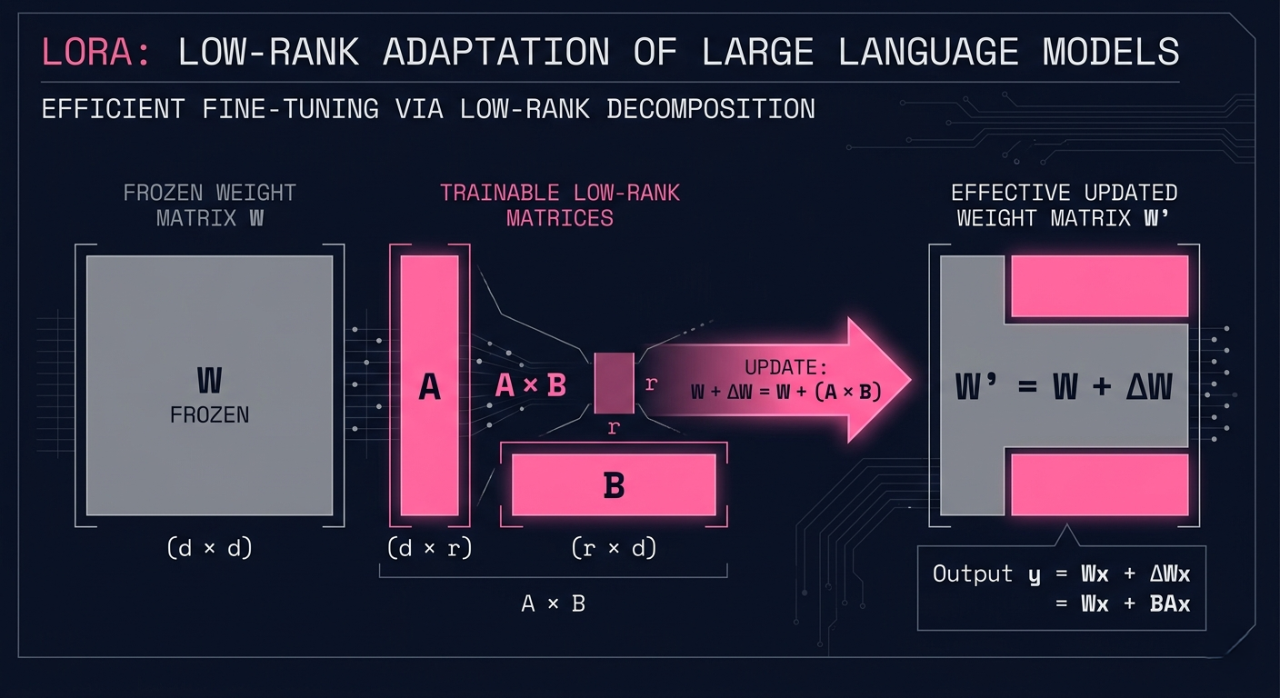
The key insight behind LoRA is that the weight changes needed to adapt a model to a new task are low-rank — they can be expressed as the product of two small matrices rather than modifying the full weight matrix. Instead of training the original weight matrix W (shape d×d), LoRA keeps W frozen and adds two small matrices A (shape d×r) and B (shape r×d) where r is much smaller than d (typically 4, 8, or 16). The effective update is W + A×B. During training, only A and B are updated. At inference time, you can either keep them separate (enabling LoRA adapters to be swapped) or merge them into the original weights.

LoRA's impact on the fine-tuning economics is dramatic. Fine-tuning a 7B parameter model with LoRA (rank 8) requires updating ~0.1% of the parameters compared to full fine-tuning. Training runs that would take weeks on expensive A100 clusters can complete in hours on a single consumer GPU. This has made fine-tuning accessible to individual researchers, small companies, and the open-source community. Every custom Stable Diffusion model you see on CivitAI, and most custom LLaMA fine-tunes, use LoRA. QLoRA (quantized LoRA) takes this further by also quantizing the frozen weights, enabling fine-tuning of 70B+ parameter models on a single GPU.

🔑 When LoRA Won't Be Enough

LoRA is excellent for style adaptation, domain-specific vocabulary, output format changes, and moderate capability improvements. It's insufficient for: teaching the model genuinely new facts (facts should go in RAG), fundamentally changing the model's reasoning architecture, or achieving capabilities that are completely absent from the base model. The low-rank assumption means LoRA can only make "small" changes to the model's behavior — it's nudging the model, not rewriting it. For large capability gaps, you need more data, higher rank, or more layers trained.

lora_training.py — Using HuggingFace PEFT

from transformers import AutoModelForCausalLM, AutoTokenizer
from peft import LoraConfig, get_peft_model, TaskType

# Load base model (frozen weights)
model = AutoModelForCausalLM.from_pretrained("meta-llama/Llama-3-8B")

# LoRA config: rank=8, apply to Q and V attention projections
config = LoraConfig(
 task_type = TaskType.CAUSAL_LM,
 r = 8, # rank — controls capacity/efficiency tradeoff
 lora_alpha = 32, # scaling factor (usually 2×-4× r)
 target_modules = ["q_proj", "v_proj"], # which layers to adapt
 lora_dropout = 0.1,
)

peft_model = get_peft_model(model, config)
peft_model.print_trainable_parameters()
# → trainable params: 4,194,304 || all params: 8,030,261,248
# → trainable%: 0.0522 ← only 0.05% of weights updated!

# After training: save just the adapter (tiny, ~16MB)
peft_model.save_pretrained("my_lora_adapter")
# Load the base model + merge adapter for inference
# peft_model.merge_and_unload() # bakes LoRA into weights

---

synthesisHow All Nine Concepts Connect

These nine concepts aren't isolated tools — they're an ecosystem. A production LLM application might use all of them simultaneously. Consider a sophisticated AI coding assistant: it uses tokenization to process both code and natural language. Its decoding uses low temperature for code generation and moderate temperature for explanations. Prompt engineering structures the system prompt with few-shot examples of good code reviews. It's an agent that can run code, search documentation, and iterate on its solutions. RAG pulls in relevant library documentation and code examples from a vector store. The model was aligned with RLHF to prefer correct, safe code over plausible-sounding but buggy code. The image/diagram generation sidebar uses a VAE latent compressor feeding a diffusion model. And the whole thing is deployed on a base model fine-tuned with LoRA on a corpus of high-quality code.

Understanding each concept in isolation is the first step. The real mastery comes from understanding which tool to reach for in which situation, and how they interact when combined. With this foundation, you can read a paper describing a new AI system and immediately map its innovations to these primitives — identifying what's genuinely new versus what's a creative recombination of familiar parts.

---

FAQFrequently Asked Questions

What is the difference between RAG and fine-tuning for adding domain knowledge? + RAG retrieves relevant information at inference time from an external knowledge store, keeping knowledge outside the model. Fine-tuning bakes knowledge into the model's weights during training. Use RAG for: frequently changing information, documents you need to cite, large knowledge bases that exceed context windows, and situations where you need provenance. Use fine-tuning for: stable specialized knowledge, specific output styles/formats, and task-specific behaviors. Most production systems use both: RAG for current facts, fine-tuning for domain-specific behavior and style. Why do LLMs sometimes produce wrong but confident-sounding answers (hallucinations)? + LLMs generate the statistically most probable continuation of a text sequence — they don't distinguish between "I know this" and "I'm making this up." When asked about something not well-represented in training data, the model generates plausible-sounding text based on patterns from related training examples. The training objective (predict the next token) rewards fluency and coherence, not factual accuracy. RAG reduces hallucination by providing retrieved evidence, but doesn't eliminate it — the model can still misinterpret retrieved passages. RLHF reduces hallucination somewhat by penalizing clearly wrong or unsupported claims if annotators catch them. What is the difference between temperature and top-P sampling? + Temperature and top-P are both methods to introduce controlled randomness into text generation, but they operate differently. Temperature scales the logits (pre-softmax scores) before computing probabilities — high temperature flattens the distribution (more uniform, more random), low temperature sharpens it (more peaked, more deterministic). Top-P (nucleus sampling) doesn't modify the distribution; instead, it builds the smallest set of tokens whose cumulative probability exceeds P and samples only from that set, discarding the very long tail of improbable tokens. In practice, both are typically used together. Temperature is the primary dial; top-P prevents the model from picking truly bizarre tokens at high temperatures. How is LoRA different from traditional fine-tuning? + Full fine-tuning updates all model parameters. For a 7B parameter model, that means storing and computing gradients for 7 billion parameters — requiring enormous GPU memory, long training runs, and large checkpoint files. LoRA keeps all original weights frozen and adds small trainable adapter matrices (A and B) to specific layers, typically the attention projection matrices. Because r (the rank) is small (4–16 in practice), the total number of trainable parameters drops by 99%+. The resulting LoRA adapter is a small file (typically 10–100MB) that can be merged into the original model or applied separately. QLoRA extends this further by quantizing the frozen weights to 4-bit precision, enabling fine-tuning of 70B models on a single 24GB GPU. What is the role of the reward model in RLHF training? + The reward model is a neural network trained to predict human preference scores for model outputs. It's trained on datasets of pairwise comparisons: human annotators see two responses to the same prompt and indicate which is better. The reward model learns to predict these preferences. During RLHF, it acts as a proxy for human judgment — the LLM generates responses, the reward model scores them, and reinforcement learning updates the LLM's weights to make higher-scored responses more probable. The reward model is critical because RL needs a differentiable signal to optimize against; you can't do RL with actual humans in the loop for every training step (too slow, too expensive). How do diffusion models generate images from text prompts? + Text-to-image diffusion models use two components together. First, a text encoder (typically CLIP) converts the prompt into an embedding vector that captures semantic meaning. Second, the diffusion model's denoising network is trained with this text embedding as conditioning — during training, it learns to denoise images while being influenced by their corresponding text descriptions. At inference, the model starts from pure noise and iteratively denoises it, at each step being guided by the text embedding. Classifier-free guidance amplifies this conditioning by computing "how much more toward the prompt" than the unconditional direction. The VAE then decodes the final latent back to pixels. What is chain-of-thought prompting and when does it help? + Chain-of-thought (CoT) prompting asks the model to explicitly output its reasoning steps before giving a final answer, either by instruction ("Think step by step") or by example (showing worked examples with intermediate reasoning). It helps significantly on multi-step reasoning tasks: math problems, logical deduction, code planning, and complex Q&A where the answer depends on correct intermediate conclusions. The likely mechanism: generating intermediate reasoning tokens gives the model additional "computation" — each token generation can attend to all previous tokens, so more explicit reasoning steps give the model more representational bandwidth for complex problems. It's less helpful for simple factual lookups or creative tasks where long reasoning chains aren't needed. What is a token context window and why does it limit LLMs? + The context window is the maximum number of tokens an LLM can process in one forward pass — including both the input (prompt, conversation history, retrieved documents) and the output being generated. This is a hard architectural constraint: the attention mechanism in a transformer attends over all tokens in the context, and the computational cost grows quadratically with context length. GPT-4 Turbo supports 128K tokens, Claude supports 200K, some models now extend to 1M+. The practical implication: very long documents, entire codebases, or long conversations eventually exceed the context window. RAG partially addresses this by retrieving relevant chunks rather than including everything.

🧬 AI Concepts Lab

Four experiments: live tokenizer, text decoding visualizer, RAG pipeline, and LoRA calculator.

Live Tokenizer (BPE approximation) Input Text Tokens (each color = one token) 0 Token count 0 Word count 0.00 Tokens/word $0.00 Est. cost (gpt-4) Token IDs Tokenizer Insights Why tokens differ from words Compare encodings Vocabulary size 50K

Larger vocabulary = fewer tokens per word, more memory for embedding table. GPT-4 uses ~100K vocab. LLaMA 3 uses ~128K.

Token probability distribution — top 15 candidates for next token

Decoding Strategy Visualizer Context Temperature 0.80 Top-P (nucleus) 0.90 Generated so far — Nucleus size — Entropy (bits)

Semantic similarity scores: query vs knowledge base chunks

RAG Pipeline Simulator User Query Top-K chunks to retrieve 3 Similarity threshold 0.60 Retrieved Chunks 0 Chunks retrieved — Best similarity

Parameter count: full fine-tuning vs LoRA

LoRA Parameter Calculator Model size (B params) 7B LoRA rank (r) 8 Target layers Q+V Hidden dimension (d) 4096 — Full fine-tune params — LoRA trainable params — % of model — VRAM saving