Neural Networks Explained: The Math Behind Machine Learning Magic

Deep Dive · 3,400 words · ~16 min read

Neural Networks Explained:
The Math Behind Machine Learning Magic

How does a computer "see" a handwritten 3? Not with magic. With 13,000 numbers, some matrix multiplication, and a clever squishing function. Here's everything — with a working lab to play with.

By The ML Deep Dive Team · April 2026 · Tags: ML, Deep Learning, Neural Nets

Table of Contents

1. The Crazy Thing Your Brain Does Effortlessly
2. What Actually Is a Neuron?
3. Layers: The Architecture of Understanding
4. Weights, Biases & Edge Detection
5. Sigmoid vs ReLU: The Squishing Function
6. The Linear Algebra Under the Hood
7. What "Learning" Actually Means
8. Getting Started: Run It Yourself
9. FAQ
10. 🧪 Interactive Lab

The Crazy Thing Your Brain Does Effortlessly

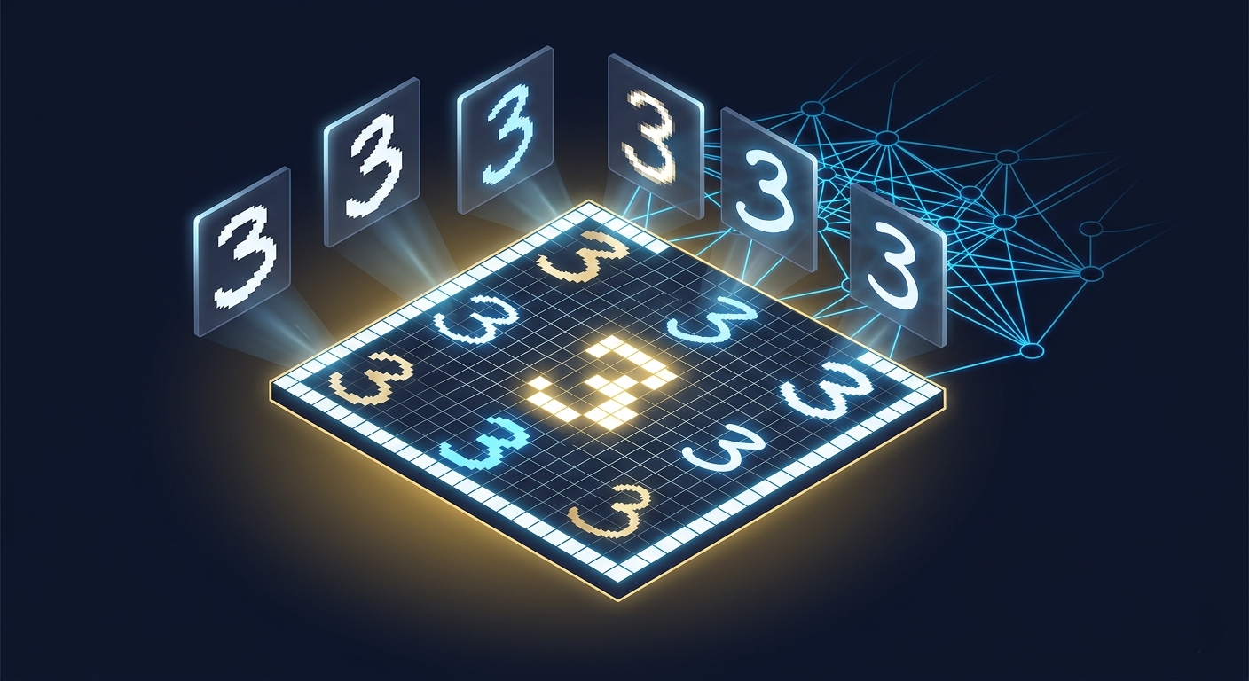
Picture this: someone scrawls a 3 on a napkin. It's lopsided. The curves don't quite meet. And it's rendered at 28×28 pixels — blurrier than a postage stamp from 1902. You glance at it for a fraction of a second and you know exactly what it is. You didn't think about it. You didn't cross-reference a mental database. Your visual cortex just… handled it.

Here's the thing most tutorials miss: the mind-bending part isn't recognizing digits — it's that every single "3" you've ever seen activated a different set of light-sensitive cells in your eye, yet somehow your brain maps all of those wildly different pixel patterns to the same concept. The specific cells that fire when you see a thick, dark 3 are completely different from the ones firing when you see a thin, loopy 3. And yet: same idea.

Now imagine someone asks you to write a program that takes a 28×28 grid of pixel values and outputs the digit it represents. Suddenly the problem transforms from trivially obvious to genuinely hard. What rules would you even write? "If there are two lumps and they're connected…"? You can feel the attempt collapse in real time. This tension — between what brains do casually and what programs struggle with — is precisely why neural networks exist.

⚡ Counterintuitive Insight

Neural networks don't "understand" digits the way you do. They learn a highly compressed mathematical function that happens to map pixel patterns to digits correctly for the training data. Understanding the difference between fitting a function and true comprehension matters enormously when these systems fail.

---

What Actually Is a Neuron?

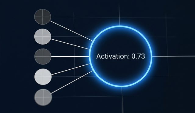
Strip away every Hollywood metaphor. Forget the biology analogies for a second. A neuron in a neural network is, at its most fundamental, a thing that holds a number between 0 and 1. That's it. It's called its activation. Think of it as a dimmer switch rather than an on/off light — not just firing or not firing, but expressing a continuous intensity.

In our digit-recognition network, the first layer of neurons maps directly to the 784 pixels in a 28×28 image. Each neuron's activation is the grayscale value of its corresponding pixel: 0 for black, 1 for white, and everything in between for shades of gray. Feed in an image of a 7, and you get 784 numbers flowing into 784 neurons. Simple, concrete, graspable.

The real analogy to keep in mind: imagine an audience at a concert. Each audience member holds up a glow stick at a brightness level proportional to how much they liked what just happened on stage. The pattern of brightness across the crowd is the information — not any individual person. That's your first layer. That pattern of activations then causes the next crowd (layer) to hold up their glow sticks, and so on, until the final row's collective brightness tells you what digit the network thinks it saw.

neuron_basics.py

# A neuron is just a number (its activation)
# Input layer: 28x28 = 784 neurons

import numpy as np
from PIL import Image

def image_to_activations(img_path):
 img = Image.open(img_path).convert('L') # grayscale
 img = img.resize((28, 28))
 pixels = np.array(img).flatten() / 255.0 # normalize 0-1
 return pixels # 784 activations

activations = image_to_activations('my_digit.png')
print(f"Input layer: {len(activations)} neurons") # → 784
print(f"Sample activation: {activations[350]:.4f}") # → e.g. 0.8235

💡 Pro Tips

Normalization is non-negotiable. Always divide pixel values by 255 before feeding them into the network. Unnormalized inputs (0–255 integers) will make training catastrophically slow or unstable because the weights will need to compensate for scale.

• Use img / 255.0, not integer division — Python 3 handles this correctly
• For real datasets, consider per-pixel mean subtraction (ImageNet-style normalization)
• Never normalize your test set using stats from your test set — use training set stats only

---

Layers: The Architecture of Understanding

Imagine you're trying to teach a toddler to recognize animals. You don't start with "this is a dog" and show them 10,000 dog photos. You first teach them about fur, then about legs, then about ears, then about snouts. Each concept is built from simpler concepts. Layers in a neural network do the same thing — except the concepts aren't named by humans; they're discovered by the training process.

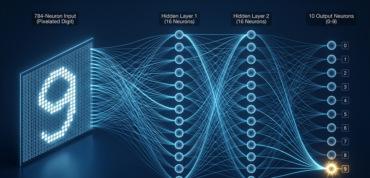
Our digit network has four layers: an input layer (784 neurons), two hidden layers (16 neurons each), and an output layer (10 neurons). The input is raw pixels. The output neurons represent digits 0 through 9 — the brightest output neuron is the network's vote. Between input and output, the hidden layers are the interesting part: they're where pixel patterns get abstracted into edges, edges into shapes, shapes into digit components.

The best hope — the ideal scenario — is that the second layer learns edges, the third layer learns loops and strokes, and the fourth layer combines those into digits. A "9" would then activate "loop at top" + "vertical line on right." Whether a real trained network actually develops such clean internal concepts is a fascinating and partially unsettled question. Sometimes it does, sometimes it develops incomprehensible, alien-looking patterns that still happen to work. That gap between our intentions and the network's learned solution is part of what makes interpretability research so important today.

✅ Why Depth Works: Layers of Abstraction

Speech recognition layers work identically: raw audio → distinct sounds → syllables → words → phrases. Computer vision: pixels → edges → textures → parts → objects. The layered hierarchy is a universal inductive bias that matches the structure of natural data surprisingly well.

---

Weights, Biases & Edge Detection

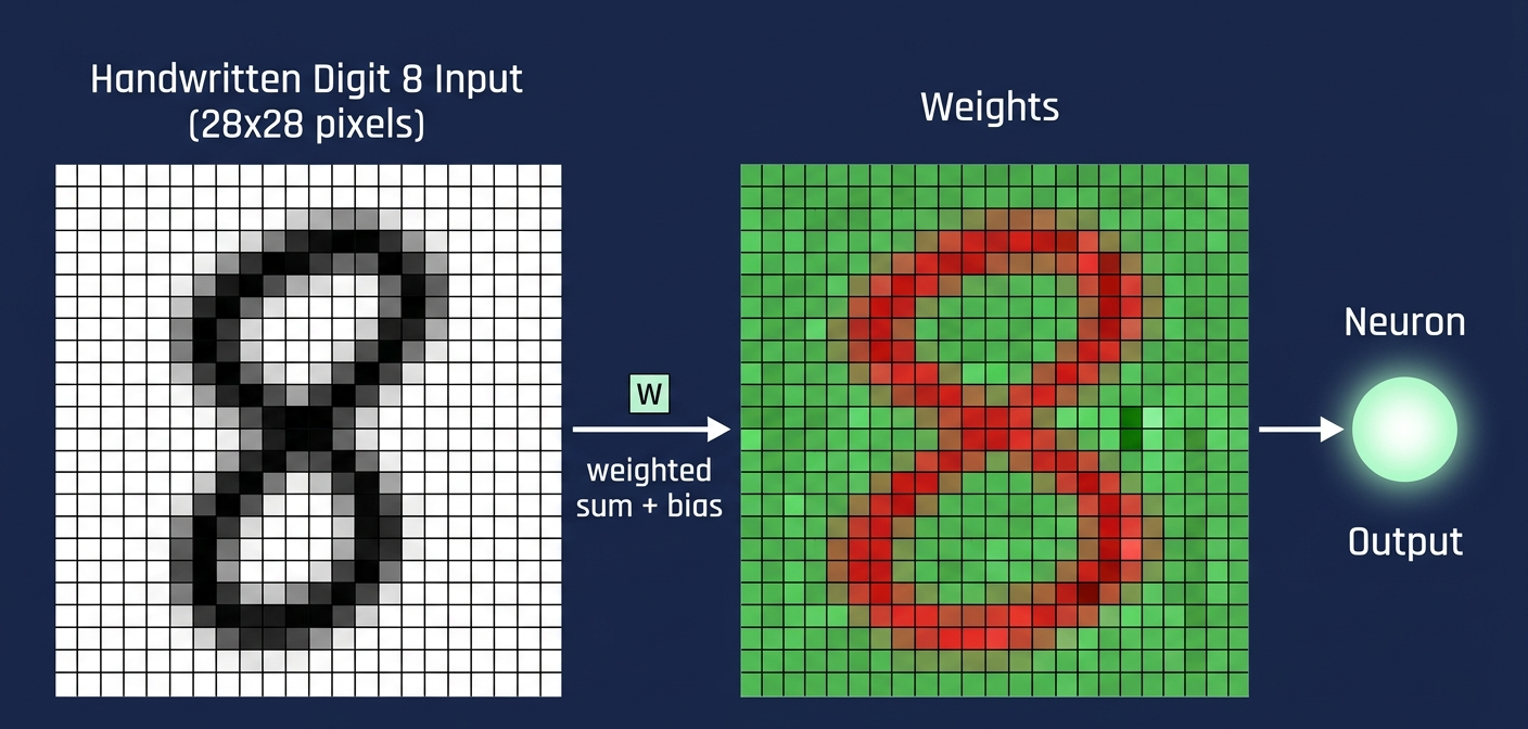
Here's where the mechanism clicks into place. Say you want one specific neuron in your hidden layer to fire when it "sees" a vertical edge in the middle of the image. How do you make that happen? You assign a weight to every connection between that neuron and every pixel in the input layer. Positive weights for pixels in the region where you want the edge, negative weights for the surrounding pixels. Then you compute the weighted sum — multiply each pixel's brightness by its weight, add them all up.

If the edge is there — bright pixels in the center column, darker on the sides — the positive terms dominate and the sum is large. If the image is uniformly gray everywhere, the positive and negative weights cancel each other out and the sum is near zero. You've encoded edge-detection logic purely through numbers.

But what if you only want the neuron to activate when there's a strong edge, not a faint one? You add a bias — a single extra number that gets added to the weighted sum before any activation function is applied. A large negative bias means the weighted sum needs to be substantially positive before the neuron lights up. A positive bias means the neuron is "eager" to activate. Weights control what pattern the neuron detects; bias controls how sensitive it is.

weighted_sum.py

# Computing activation for one hidden neuron

def neuron_activation(inputs, weights, bias, activation_fn):
 """
 inputs: array of shape (784,) — pixel activations
 weights: array of shape (784,) — one weight per connection
 bias: scalar — threshold shift
 """
 weighted_sum = np.dot(inputs, weights) + bias
 return activation_fn(weighted_sum)

# Edge detection weights: positive center, negative surround
weights = np.zeros(784)
weights[350:378] = 1.0 # center column — positive
weights[322:350] = -0.5 # left column — negative
weights[378:406] = -0.5 # right column — negative
bias = -5.0 # only fires on strong edges

⚠️ Common Mistakes

• Initializing all weights to zero: Every neuron learns the same thing. Use random initialization (Xavier/He init).
• Forgetting biases entirely: Without bias, your decision boundary must pass through the origin — massively limits expressiveness.
• Making weights too large at init: Causes exploding gradients during training. Keep initial weights small (e.g., normal distribution with std ~0.01).

---

Sigmoid vs ReLU: The Squishing Function

The weighted sum of 784 inputs with weights that can be positive or negative can produce any real number — positive or negative, potentially enormous. But we need neuron activations to sit between 0 and 1 (or at least be bounded). Enter the activation function: a mathematical wrapper that takes an arbitrary number and squishes it into a useful range.

The classic choice is the sigmoid function (also called the logistic curve): σ(x) = 1 / (1 + e^{-x}). Very negative inputs → output near 0. Very positive inputs → output near 1. Around zero → smooth transition. It's elegant, motivated by a biological analogy of neurons being "mostly off" or "mostly on", and it was the default for decades.

Then researchers discovered something humbling: sigmoid is actually pretty bad for training deep networks. The gradients (the signals that tell weights how to adjust during learning) tend to vanish as they propagate backwards through many sigmoid layers — the so-called vanishing gradient problem. The fix? The ReLU (Rectified Linear Unit): ReLU(x) = max(0, x). Brutally simple. If the input is negative, output zero. If positive, pass it through unchanged. This keeps gradients alive across many layers and makes training dramatically faster. Modern networks almost universally use ReLU or one of its variants (Leaky ReLU, GELU, SiLU). Sigmoid still appears — but usually only in the output layer for binary classification tasks.

activation_functions.py

import numpy as np

# Sigmoid — classic but vanishes in deep nets
def sigmoid(x):
 return 1 / (1 + np.exp(-x))

# ReLU — fast, modern, gradient-friendly
def relu(x):
 return np.maximum(0, x)

# Leaky ReLU — avoids "dying ReLU" problem
def leaky_relu(x, alpha=0.01):
 return np.where(x > 0, x, alpha * x)

# Comparing outputs for x = [-2, 0, 2, 5]
x = np.array([-2, 0, 2, 5])
print("Sigmoid:", sigmoid(x)) # [0.119, 0.5, 0.880, 0.993]
print("ReLU: ", relu(x)) # [0, 0, 2, 5 ]

💡 The Myth About Biological Realism

ReLU won not because it's more biologically accurate — it's arguably less biologically realistic. It won because it works better in practice. This is a recurring theme in deep learning: the "right" solution is empirical, not theoretical. The field is still working out why ReLU works so well.

---

The Linear Algebra Under the Hood

Writing out "weighted sum of 784 activations with 784 weights plus a bias, then apply sigmoid" for every neuron individually is both verbose and slow. There's a much cleaner way — and it's not just notation sugar; it unlocks orders-of-magnitude speedups via GPU parallelism.

Stack all 784 input activations into a column vector a. Arrange all the weights for the hidden layer into a matrix W, where each row represents the weights for one hidden neuron. Then the entire weighted-sum computation for all 16 hidden neurons at once is just: Wa + b, where b is the bias vector. Wrap in the activation function and you get the full layer transition: σ(Wa + b). Four symbols. Elegant.

This is why understanding linear algebra is so essential in ML — not as abstract math, but as the actual language the computation is written in. Matrix-vector multiplication maps directly to highly optimized CUDA kernels. Libraries like NumPy, PyTorch, and JAX make this as fast as the hardware physically allows. That little expression σ(Wa + b) is, in a very real sense, the atomic unit of all modern deep learning.

layer_forward.py

import numpy as np

class DenseLayer:
 def __init__(self, in_size, out_size):
 # Xavier initialization — prevents vanishing/exploding gradients
 self.W = np.random.randn(out_size, in_size) * np.sqrt(2/in_size)
 self.b = np.zeros(out_size)

 def forward(self, a):
 # σ(Wa + b) — the fundamental operation
 z = self.W @ a + self.b # matrix-vector product + bias
 return np.maximum(0, z) # ReLU activation

# Full network: 784 → 16 → 16 → 10
layers = [
 DenseLayer(784, 16),
 DenseLayer(16, 16),
 DenseLayer(16, 10),
]

def forward_pass(x):
 a = x
 for layer in layers:
 a = layer.forward(a)
 return a # 10-dimensional output vector

💡 Parameter Count Reality Check

A "simple" network with layers [784, 16, 16, 10] has exactly 12,960 parameters:

• 784×16 + 16 = 12,560 (layer 1)
• 16×16 + 16 = 272 (layer 2)
• 16×10 + 10 = 170 (layer 3)

GPT-4 is estimated to have ~1.8 trillion parameters. Same math. Wildly different scale.

---

What "Learning" Actually Means

When people say a neural network "learned to recognize digits," they mean the computer found values for all 12,960 weights and biases such that when you run any digit image through the forward pass, the correct output neuron tends to be the brightest. That's it. Learning = finding good numbers. The process of finding them is called gradient descent with backpropagation, and it's the subject of the next video in this series.

Here's a thought experiment: imagine sitting down to set all 12,960 weights manually. You'd want layer 1 weights to detect edges. Layer 2 weights to detect curves and loops. Layer 3 to combine them into digits. You could do this — and it would probably work, partially. This exercise isn't just hypothetical. It's a form of network interpretability: understanding what each weight actually encodes is how you debug a network that's failing, and how you build trust in one that's succeeding. The black-box framing ("just train it and trust it") leads to nasty surprises.

The counterintuitive truth about learning in neural networks: the network doesn't "understand" edges and loops the way we hope it does. It finds whatever mathematical surface best separates the training examples, which often looks like the features we expect, but sometimes looks alien and incomprehensible. Modern interpretability research (mechanistic interpretability) is actively trying to reverse-engineer what concepts these weights actually encode.

⚠️ The Danger of the Black Box

A network that achieves 99% accuracy on your test set might be detecting watermarks in the training images, correlations with paper texture, or other spurious signals. Always test on truly out-of-distribution data before trusting a model for anything consequential.

---

Getting Started: Run It Yourself in 5 Minutes

Enough theory. Here's how to have a live digit-recognizing neural network running on your machine, using PyTorch and the MNIST dataset. Every line does exactly what you've read about above — you'll recognize the math instantly.

Step 1: Install dependencies

# Python 3.9+ recommended
pip install torch torchvision matplotlib numpy

Step 2: train_mnist.py — the full network

import torch
import torch.nn as nn
from torchvision import datasets, transforms

# Step 1: Load MNIST data
transform = transforms.ToTensor()
train_data = datasets.MNIST(root='.', train=True,
 download=True, transform=transform)
loader = torch.utils.data.DataLoader(train_data,
 batch_size=64, shuffle=True)

# Step 2: Define the network — 784 → 16 → 16 → 10
model = nn.Sequential(
 nn.Flatten(), # 28x28 → 784
 nn.Linear(784, 16), # Wa + b for 16 neurons
 nn.ReLU(), # activation
 nn.Linear(16, 16),
 nn.ReLU(),
 nn.Linear(16, 10), # 10 output neurons
)

# Step 3: Training loop
optimizer = torch.optim.Adam(model.parameters(), lr=1e-3)
loss_fn = nn.CrossEntropyLoss()

for epoch in range(5):
 for X, y in loader:
 pred = model(X)
 loss = loss_fn(pred, y)
 optimizer.zero_grad()
 loss.backward() # backpropagation
 optimizer.step() # update weights & biases
 print(f"Epoch {epoch+1} loss: {loss.item():.4f}")

Run this and you'll see the loss drop from ~2.3 (random chance) to ~0.15 within 5 epochs. The network has found 12,960 numbers that collectively solve the digit recognition problem — without you writing a single explicit rule.

How It All Connects

Let's map the journey: a 28×28 image becomes 784 activation values (the input layer). A weight matrix transforms those into 16 hidden neuron activations (edge detectors, ideally). Another weight matrix compresses those into 16 higher-level activations (curve/loop detectors). A final matrix produces 10 output activations, one per digit. The brightest wins. Every step is just: multiply by weights, add bias, apply activation function. Repeated three times.

"Learning" means running 60,000 training examples through this pipeline, measuring how wrong the outputs are, and using calculus (backpropagation) to nudge all 12,960 parameters in the direction that reduces the error. The network never sees an explicit rule. It discovers the structure of digits entirely through gradient descent on a loss function. That's the miracle, and that's why it generalizes — not perfectly, but remarkably well.

---

Frequently Asked Questions

Why 16 neurons in the hidden layers? Is that optimal? 16 is not optimal — it's a convenient number. The architecture (number of hidden layers and neurons per layer) is a hyperparameter you choose before training. Too few neurons and the network can't represent the complexity of the problem (underfitting). Too many and it memorizes the training data without generalizing (overfitting). Finding the right size is part empirical, part art form. For MNIST, even 16 neurons gets you to ~97% accuracy. CNNs (convolutional neural networks) can hit >99.7% by exploiting the spatial structure of images. What's the difference between a weight and a parameter? "Parameters" is the umbrella term for everything the network learns: weights and biases both count as parameters. "Weights" specifically refer to the values on connections between neurons. Biases are the additive offsets. When people say "GPT-3 has 175 billion parameters," they mean all weights and biases across all layers combined. Why does sigmoid cause vanishing gradients but ReLU doesn't? The gradient of the sigmoid function maxes out at 0.25 (at x=0) and approaches 0 for large positive or negative inputs. When you multiply many of these small gradients together during backpropagation across many layers, the signal essentially disappears. ReLU has a gradient of exactly 1 for all positive inputs — no shrinkage. For negative inputs, the gradient is 0 (the "dead neuron" problem), which Leaky ReLU addresses by using a small slope (e.g., 0.01) instead of hard 0. Does the network actually learn edge detectors in its first hidden layer? For simple fully-connected networks like ours, the answer is: sometimes, partially, and not cleanly. CNNs are much better at this because their architecture explicitly forces spatial locality (each neuron only sees a small patch). When researchers visualize the learned weights of CNN filters, they often see clean edge detectors, color blobs, and texture patterns in early layers. For fully-connected networks, the relationship is messier. How do I know if my network is overfitting? Track two metrics: training loss (how wrong the network is on examples it's seen) and validation loss (on examples it hasn't seen). If training loss decreases but validation loss increases, you're overfitting. Remedies include: using more training data, adding dropout layers, reducing network size, or regularization (L1/L2 penalties on weights). What is backpropagation doing at a high level? Backpropagation is the algorithm that efficiently computes how much each weight contributed to the current error. It works by propagating the gradient of the loss function backwards through the network using the chain rule of calculus. Once you know how much each weight contributed to the error, gradient descent adjusts them all in the direction that reduces the error. The full mathematical treatment is the subject of the next post in this series. Can this simple network generalize to images it's never seen? Yes — that's the point of the train/test split. A well-trained network on MNIST achieves ~97–98% accuracy on a held-out test set it has never seen. However, feed it an image of a digit written in an unusual style, at a rotation, or with noise artifacts, and accuracy drops sharply. This brittleness is why CNNs with data augmentation (rotations, shifts, noise) dramatically outperform plain fully-connected networks on real-world handwriting. Is this the same math used in large language models like GPT? The fundamental operations are identical: matrix-vector products, bias additions, activation functions, and gradient descent. What's different is the architecture: LLMs use transformer blocks with attention mechanisms, not simple dense layers. But every attention operation is ultimately implemented through the same linear algebra. Understanding the simple network described here is genuinely prerequisite to understanding transformers.

🧪 Interactive Neural Network Lab

Tweak every parameter. Watch the network respond in real time. Draw a digit, then change the architecture and see how it affects the output signal.

12,960 Total Parameters 4 Layers ReLU Activation Fn ? Prediction

Draw a Digit

Draw here (28×28 mapped)

Architecture

Hidden Layer 1 Neurons 16 Hidden Layer 2 Neurons 16 Activation Function

Signal Parameters

Input Noise Level 0.00 Weight Scale (init) 1.0× Global Bias Shift 0.0

Actions

Output Activations