Multi-Layer Perceptrons: Where LLMs Hide Their Knowledge

Where Facts Live in Neural Networks Part 6

MLP blocks, neurons & superposition Multi-Layer
Perceptrons:
Where LLMs Hide Their Knowledge

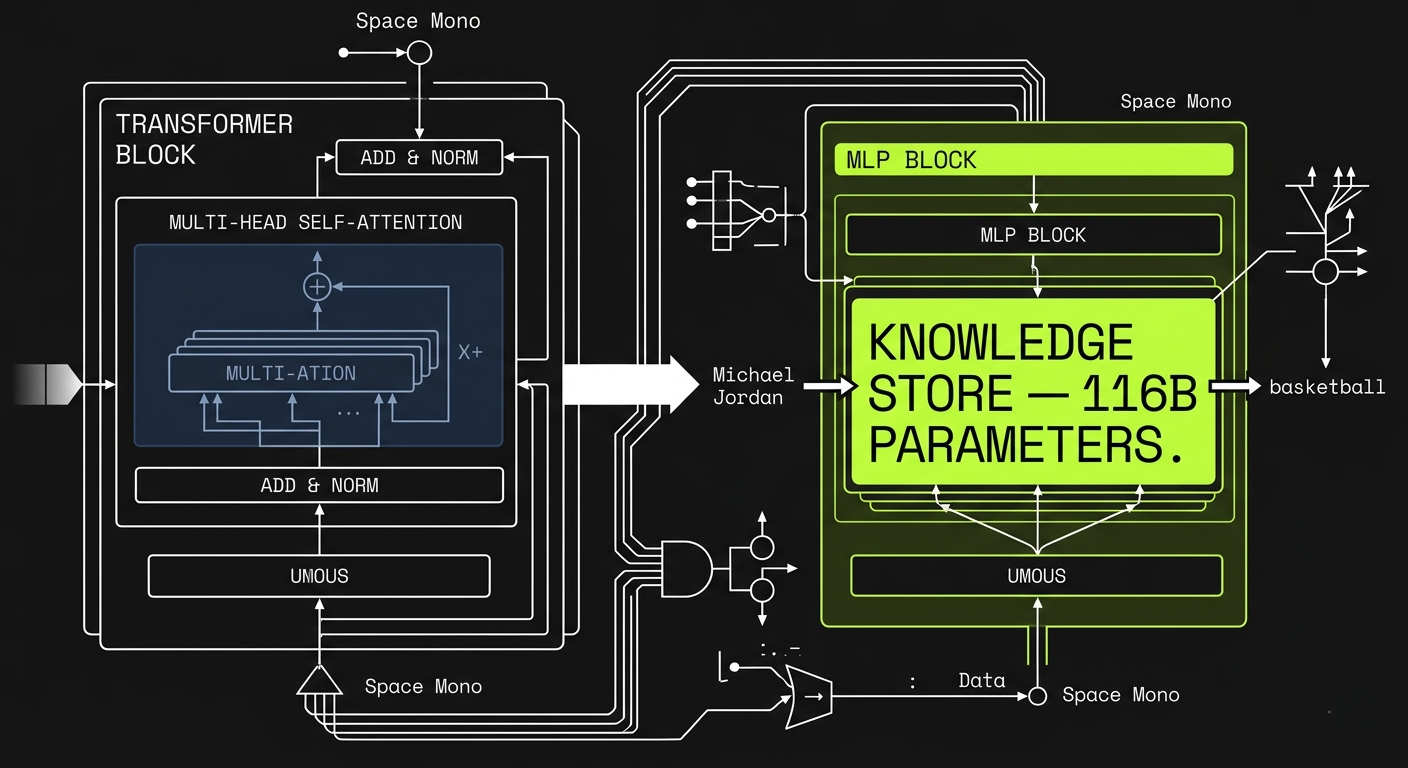
How does GPT know Michael Jordan plays basketball? The answer lives in MLP blocks — two matrix multiplications, a ReLU, and 116 billion parameters that form the model's "knowledge memory." Here's exactly how it works.

Read the Deep Dive ↓ Open the Lab ⚗️ Table of Contents

1. Where Facts Actually Live
2. MLP Structure: Two Matrices, One ReLU
3. The Up-Projection: Asking Questions
4. ReLU as an AND Gate
5. Down-Projection: Retrieving Knowledge
6. Parameter Count: 116 of 175 Billion
7. Superposition: The Dimension Explosion
8. Getting Started: Inspect Real MLPs

01Where Facts Actually Live in a Language Model

Here's a question that sounds simple but turns out to be surprisingly hard to answer: when you ask ChatGPT "what sport does Michael Jordan play?" and it correctly responds "basketball" — where exactly in those 175 billion numbers does that fact reside? It's not a database lookup. It's not a search. It's a forward pass through matrices. So which matrices? Which layers? Which neurons?

Researchers at Google DeepMind have been probing exactly this question, and their early results point clearly in one direction: facts appear to be stored primarily in the MLP (Multi-Layer Perceptron) blocks of the transformer. Not in the attention blocks, which handle routing and contextual updating. Not in the embedding matrices. The MLPs — sometimes dismissed as the "boring" part of the architecture next to the elegant attention mechanism — turn out to be the actual knowledge store of large language models.

Here's the thing most tutorials miss: attention blocks and MLP blocks have fundamentally different roles. Attention routes information — it figures out which tokens should influence which others. MLP blocks store and retrieve information — they apply learned transformations that encode facts, relationships, and world knowledge baked in from training. The analogy that resonates is RAM versus hard disk. Attention moves data around working memory; MLPs are the persistent storage that training wrote to. And there's much more storage than most people realize.

Key Insight: 2/3 of Parameters Live in MLPs

In GPT-3, the MLP blocks account for approximately 116 billion of the 175 billion total parameters — around 66%. Attention blocks account for ~58 billion, with the rest in embeddings and normalization. Despite attention getting all the theoretical glory, the majority of the model's "brain" by raw parameter count is in these relatively simple matrix-multiplication blocks. Understanding MLPs is understanding where the model actually learned its knowledge.

---

02MLP Structure: Two Matrices and One Surprisingly Powerful ReLU

Strip away everything else and the MLP block is almost shockingly simple. A vector flows in — say, the embedding for the second token in "Michael Jordan," which attention has already enriched with information about both names. That vector gets multiplied by a big matrix (the up-projection), gets passed through ReLU, gets multiplied by another big matrix (the down-projection), and the result gets added back to the original vector. That's it. No attention pattern computation. No softmax. No cross-token communication. Pure feedforward.

The crucial detail: each token's vector goes through this independently and in parallel. The vectors don't talk to each other during MLP processing — contrast this with attention, where every token can influence every other token. This independence is both a constraint and an advantage. The constraint means MLP blocks can only process one token's context at a time. The advantage means the computation is embarrassingly parallelizable across the entire context window simultaneously — every token runs its MLP pass at the same time.

Imagine you're the MLP block processing the embedding vector for "Jordan." You receive a rich vector that encodes, through attention's earlier work: "the token 'Jordan', preceded by 'Michael', so together this represents the person Michael Jordan." Your job is to apply whatever transformations are needed to prepare this vector for predicting the next word. In our fact-storage model, that means detecting the Michael Jordan pattern and adding "basketball" information to the vector. The two matrix multiplications and one nonlinearity accomplish this in three elegant steps.

Warning: MLP ≠ "Simple" at Scale

The word "simple" applied to MLPs can be misleading. Yes, the mathematical operation is straightforward: two matrix multiplications with a nonlinearity. But at GPT-3 scale, that "simple" operation involves a matrix with 12,288 columns and ~49,152 rows — multiplying a 12,288-dimensional vector against this produces a 49,152-dimensional intermediate representation. The simplicity is in the computational pattern; the richness is in what these enormous matrices have learned to encode over months of training on hundreds of billions of tokens.

mlp_forward.py

import torch
import torch.nn as nn

class MLP(nn.Module):
 """
 One MLP block in a GPT-style transformer.
 The entire 'fact storage' mechanism boils down to this.
 """
 def __init__(self, d_model=12288, expansion=4):
 super().__init__()
 d_ff = d_model * expansion # 49,152 in GPT-3

 # Up-projection: "asks 49,152 questions"
 self.W_up = nn.Linear(d_model, d_ff, bias=True)
 # Down-projection: "retrieves answers"
 self.W_down = nn.Linear(d_ff, d_model, bias=True)
 # Activation: ReLU (clip negatives) or GELU (smooth version)
 self.act = nn.ReLU() # conceptually; GPT uses GELU

 def forward(self, x):
 # x: (batch, seq, d_model) — independent per token
 h = self.W_up(x) # → (batch, seq, d_ff)
 h = self.act(h) # → zero out negatives
 h = self.W_down(h) # → (batch, seq, d_model)
 return x + h # residual connection

# GPT-3 MLP parameter count per block:
d_model, d_ff = 12288, 49152
params_per_mlp = 2 * d_model * d_ff # W_up + W_down
print(f"{params_per_mlp/1e9:.2f}B params per MLP block")
# → 1.21B params per MLP block × 96 layers = 116B total

---

03The Up-Projection: A Matrix That Asks 49,152 Questions Simultaneously

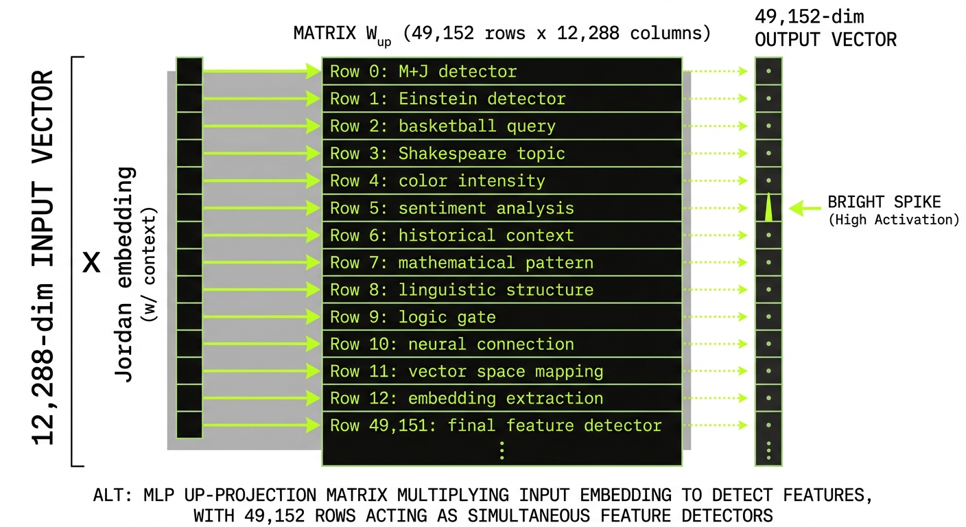
The first step of the MLP block is to multiply the input embedding by the up-projection matrix W_up. Think of each row in this matrix as a question being asked of the input vector. The dot product between that row and the input vector tells you how well the input matches what that row is "looking for." If a row encodes the direction corresponding to "first name Michael + last name Jordan," then the dot product would be high for an input vector representing Michael Jordan and near zero for anything else.

In GPT-3, this matrix has 49,152 rows — four times the embedding dimension of 12,288. That's 49,152 simultaneous questions being asked of every input vector. Some of these rows might detect grammatical patterns. Some might detect semantic relationships. Some might detect specific named entities — maybe one row fires strongly for "Michael Jordan," another for "Albert Einstein," another for "Paris France," and so on. The bias vector added after this multiplication acts as a threshold: you add a negative bias to require that the match be strong enough before the neuron fires.

The up-projection's critical function is feature detection combined with threshold gating. The result is a 49,152-dimensional intermediate vector where each component says "how much does this input match the feature I'm detecting?" A component of 2 means strong match. A component of -1 means no match or anti-match. This intermediate representation is about to get filtered by ReLU to create a clean binary-ish gate — but first, notice the richness here. A single vector has been simultaneously matched against 49,152 learned feature detectors in one matrix multiplication.

The "AND Gate" Intuition

If a row in the up-projection matrix equals the direction "Michael + Jordan" (their vectors summed), then the dot product with an input vector that encodes both names equals 2 (one for each name), but an input encoding only "Michael" (first name only) gives 1, and an input encoding "Alexis Jordan" or "Michael Phelps" also gives 1. Add a bias of -1, and you get: Michael Jordan → 1 (positive, fires), anyone else → 0 or negative (doesn't fire). That's an AND gate implemented as a linear operation plus bias plus threshold. Clean and elegant.

up_projection.py

import numpy as np

# Toy example: d_model=3, d_ff=4
# Suppose directions exist:
first_michael = np.array([1, 0, 0]) # "first name Michael"
last_jordan = np.array([0, 1, 0]) # "last name Jordan"
basketball = np.array([0, 0, 1]) # "basketball"

# Row 0 of W_up: "Michael AND Jordan" detector
W_up_row0 = first_michael + last_jordan # [1,1,0]
bias_0 = -1 # threshold: need sum > 1 to fire

# Test different inputs
test_cases = {
 "Michael Jordan": np.array([1, 1, 0]), # both names
 "Michael only": np.array([1, 0, 0]), # first name only
 "Alexis Jordan": np.array([0, 1, 0]), # last name only
 "Random person": np.array([0, 0, 0]), # unrelated
}

for name, vec in test_cases.items():
 score = np.dot(W_up_row0, vec) + bias_0
 print(f"{name:18s}: score = {score:+.1f} → fires: {score > 0}")
# Michael Jordan : score = +1.0 → fires: True ✓
# Michael only : score = 0.0 → fires: False
# Alexis Jordan : score = 0.0 → fires: False
# Random person : score = -1.0 → fires: False ✓

---

04ReLU as an AND Gate: The Elegant Nonlinearity

After the up-projection produces a 49,152-dimensional vector, it gets passed through ReLU — the Rectified Linear Unit. ReLU's definition is almost insultingly simple: if the input is positive, pass it through unchanged. If it's negative, clip it to zero. That's the entire function: max(0, x). One line. No parameters. No learning. And yet this trivial operation is what makes the MLP block capable of implementing genuine boolean logic.

Here's why the bias in the up-projection matters so much. Without the -1 bias in our Michael Jordan example, a vector encoding only "Michael" (first name) would produce a score of +1 for our AND-gate neuron — it would fire for any Michael, not just Michael Jordan. Adding the bias of -1 shifts the threshold: you need a score of +2 to fire (which only full-name Michael Jordan produces), and anything less becomes 0 or negative. ReLU then clips all those zeros and negatives cleanly to zero. The result: a neuron that activates if and only if the input represents Michael Jordan.

Models like GPT-3 actually use GELU (Gaussian Error Linear Unit) rather than pure ReLU. GELU has the same basic shape but is smoother near zero — it doesn't have a hard kink at x=0, which makes training slightly more stable. The conceptual picture is identical: positive values pass through, negative values get suppressed. For building intuition, think ReLU; for production implementations, it's GELU. The AND-gate behavior emerges from both.

Myth: Neural Network "Neurons" Are Inspired By Biology

When people say "transformer neurons" they're referring to these post-ReLU values. Terminology aside, these have little biological resemblance. Real neurons have complex dendritic computations, spike timing, neuromodulation, and spatial structure. The "neuron" in an MLP is just a scalar value: a weighted sum passed through a clipping function. The biological analogy was motivating in 1943 (the McCulloch-Pitts model). In 2024, it's best treated as historical metaphor rather than mechanistic truth.

relu_gelu_compare.py

import numpy as np

def relu(x): return np.maximum(0, x)

def gelu(x):
 """GELU: smooth approximation of ReLU, used in GPT."""
 return 0.5 * x * (1 + np.tanh(
 np.sqrt(2/np.pi) * (x + 0.044715 * x**3)
 ))

# AND gate behavior: fires only for Michael Jordan
scores = {
 "Michael Jordan": 1.0, # up-proj score + bias
 "Michael Phelps": 0.0, # only first name matches
 "Alexis Jordan": 0.0, # only last name matches
 "LeBron James": -1.0, # neither matches
}

print("Name ReLU GELU")
for name, s in scores.items():
 print(f"{name:18s} {relu(s):.3f} {gelu(s):.3f}")
# Michael Jordan 1.000 0.841 ← fires!
# Michael Phelps 0.000 0.000 ← silent
# Alexis Jordan 0.000 0.000 ← silent
# LeBron James 0.000 -0.000 ← silent

---

05Down-Projection: Reading the "Answer" Out of Neurons

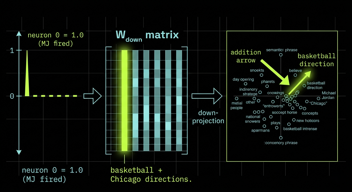
After the ReLU creates a sparse, clipped intermediate vector, the second matrix multiplication maps it back down to the embedding dimension. This is the down-projection, W_down. If the up-projection asked questions, the down-projection reads the answers. And the cleanest way to understand it is to think column-by-column rather than row-by-row.

Each column in W_down is a vector in the full embedding space — 12,288 dimensions. It represents "what should be added to the output when the corresponding neuron fires." If neuron 0 (our Michael Jordan detector) is active with a value of 1.0, then column 0 of W_down gets added to the output with weight 1.0. If neuron 0 is inactive (value 0 after ReLU), column 0 contributes nothing. In our toy example, if column 0 points in the "basketball" direction in embedding space, then: Michael Jordan input → neuron 0 fires → basketball direction added to output. Fact retrieved.

The power here is in the combination. A single neuron can write to multiple semantic directions through its column — not just basketball, but maybe also "athletic excellence," "Nike sponsorship," "Chicago," and "1990s NBA" all packed into one column as a multi-directional addition to the output embedding. And simultaneously, the final output is a sum of all active neurons' columns. The MLP's output is therefore a rich, fact-informed update to each token's embedding — potentially containing dozens of associated facts retrieved in parallel through many different neurons firing simultaneously.

Common Mistake: Thinking One Neuron = One Fact

It's tempting to imagine a "Michael Jordan neuron" — one specific neuron that represents exactly and only that fact. Real models almost never work this way. The evidence strongly suggests neurons are polysemantic: a single neuron activates for multiple unrelated concepts (maybe "Michael Jordan" AND "Leonardo da Vinci" AND "basketball courts" all activate neuron 4,721 to some degree). This is the superposition phenomenon, and it's why mechanistic interpretability is hard. Don't expect a clean one-to-one mapping between neurons and facts.

down_projection.py

import numpy as np

# Toy down-projection: d_ff=4 neurons, d_model=3
# Each column = "what to add if this neuron fires"
basketball_dir = np.array([0,0,1]) # "basketball" in embedding space
chicago_dir = np.array([0.5,0,0])# "Chicago" in embedding space

# Column 0: what to add when MJ neuron fires
# Encodes: basketball + Chicago (multiple facts at once!)
W_down_col0 = basketball_dir + chicago_dir

# Simulate: neuron 0 fires (MJ detected), rest silent
neuron_values = np.array([1.0, 0.0, 0.0, 0.0]) # after ReLU

# W_down is (d_ff=4 rows) x (d_model=3 cols), think column-by-column
W_down = np.array([W_down_col0, [0,0,0], [0,0,0], [0,0,0]]).T

# The output: weighted sum of columns by neuron values
delta_e = W_down @ neuron_values
print("Update to embedding:", delta_e)
# → [0.5, 0.0, 1.0] — encodes Chicago + basketball
# This gets ADDED to the original "Jordan" embedding
# Result: embedding now encodes Michael Jordan + basketball + Chicago

---

06Parameter Count: How MLP Blocks Dominate GPT-3's 175 Billion

Let's run the GPT-3 numbers. The up-projection matrix W_up has 49,152 rows (4 × 12,288) and 12,288 columns — that's 49,152 × 12,288 = approximately 604 million parameters. The down-projection matrix W_down has the transposed dimensions, also 604 million. Together, one MLP block has about 1.2 billion parameters. GPT-3 has 96 MLP blocks. Multiply: 96 × 1.2B ≈ 116 billion parameters in MLP blocks alone.

Adding this to what we've accumulated — about 58 billion in attention heads and about 1.2 billion in embeddings — brings us to approximately 175 billion, as advertised. The attention blocks, despite being conceptually central to the transformer architecture, account for only about a third of the parameters. The MLP blocks account for two-thirds. The normalization layers and bias vectors make up the remainder, a trivially small fraction.

This distribution has a clear implication for where training compute goes. Every backpropagation pass through GPT-3 adjusts 116 billion MLP parameters — the weights that encode world knowledge, facts, relationships, and learned patterns. The attention parameters (58B) handle the contextual routing. The embedding parameters handle the token-to-vector mapping. If you want to understand why these models "know" so much, the answer is that those 116 billion MLP parameters are doing the heavy lifting of knowledge storage.

The 4x Expansion Factor Is a Design Choice

Why 4× expansion in the MLP hidden dimension? It's not derived from theory — it's empirical. Researchers found that 4× provided a good balance between representational power and computational cost. Some modern architectures use different ratios (LLaMA uses ~2.7× with SwiGLU activation, which has an implicit gating mechanism). The key constraint is hardware efficiency: the matrices need to fit cleanly in GPU memory and be shaped for optimal BLAS operations. The "magic number" is as much engineering as science.

---

07Superposition: The Geometric Miracle That Makes LLMs Scale

Here's the most mind-bending concept in this entire series: high-dimensional spaces can store far more information than their nominal dimensionality suggests. This isn't obvious. In 3D space, you can have at most 3 mutually perpendicular vectors. In 12,288D space, you can have exactly 12,288 perfectly perpendicular directions. So if information is encoded as orthogonal directions in embedding space, the maximum number of independent facts you can represent is capped by the dimensionality. Right?

Wrong — if you relax the perpendicularity constraint just a little. A consequence of the Johnson-Lindenstrauss lemma is that the number of nearly perpendicular vectors you can fit into a d-dimensional space grows exponentially with d. Not linearly — exponentially. If you allow directions to be 89-91 degrees apart (rather than exactly 90), a 100-dimensional space can hold not 100 but something like 10,000 or 100,000 nearly-perpendicular vectors. At 12,288 dimensions, the number is astronomical. This is the superposition hypothesis: models might encode many more features than dimensions by representing features as near-orthogonal directions, with some tolerated "crosstalk" noise between them.

The consequence for interpretability is significant. If individual features are represented as superpositions of many neurons rather than single neurons, then looking at "which neuron fired" doesn't tell you which feature was activated. You'd need to look at the pattern across many neurons simultaneously. This is exactly what sparse autoencoders are designed to do — they learn to decompose the superimposed neuron activations back into interpretable individual features. Anthropic, DeepMind, and others are actively publishing on this. Mechanistic interpretability is one of the most exciting frontiers in AI safety research precisely because understanding what features are encoded in these models is essential for knowing what they've actually learned.

Counterintuitive: More Dimensions = Exponentially More "Space"

Most people's intuition about dimensions comes from 2D and 3D geometry. In those spaces, you can only fit 2 or 3 orthogonal vectors, and near-orthogonal doesn't gain you much. But high-dimensional geometry is genuinely alien: in 100+ dimensions, almost all random pairs of vectors are nearly perpendicular. The curse of dimensionality is actually a gift for representation: the exponential growth in near-orthogonal vectors means a 12,288-dimensional space can represent astronomically more independent concepts than 12,288. This partially explains why scaling model size gives such dramatic capability improvements — each new dimension added contributes exponentially to representational capacity.

superposition_demo.py

import numpy as np
import matplotlib.pyplot as plt

def nearly_perpendicular_vectors(n_dims, n_vecs, iterations=5000):
 """
 Iteratively nudge n_vecs random vectors to be nearly orthogonal
 in n_dims dimensional space. Returns final angle distribution.
 """
 vecs = np.random.randn(n_vecs, n_dims)
 # Normalize to unit vectors
 vecs /= np.linalg.norm(vecs, axis=1, keepdims=True)

 lr = 0.01
 for _ in range(iterations):
 dots = vecs @ vecs.T # all pairwise dot products
 np.fill_diagonal(dots, 0) # ignore self-similarity
 grad = 2 * dots @ vecs # push apart
 vecs -= lr * grad
 vecs /= np.linalg.norm(vecs, axis=1, keepdims=True)

 # Measure angles between all pairs
 final_dots = vecs @ vecs.T
 mask = np.triu(np.ones_like(final_dots, dtype=bool), k=1)
 angles = np.degrees(np.arccos(np.clip(final_dots[mask], -1, 1)))
 return angles

# In 100D space, fit 10,000 vectors (100× oversubscription)
angles = nearly_perpendicular_vectors(n_dims=100, n_vecs=10000)
print(f"All angles in range: {angles.min():.1f}° to {angles.max():.1f}°")
# → All angles in range: 88.9° to 91.1° — nearly orthogonal!
print(f"Stored {len(vecs)} vectors in {100}D space (ratio: {10000/100}×)")
# → Stored 10000 vectors in 100D space (ratio: 100×)

---

08Getting Started: Inspect Real MLP Neurons With TransformerLens

The best way to feel the MLP internals is to hook into a real model and watch neurons fire. TransformerLens by Neel Nanda (yes, the DeepMind researcher from the video) is the cleanest library for this — it gives you surgical access to intermediate activations with minimal boilerplate.

inspect_mlp.py

# pip install transformer-lens
import transformer_lens as tl

# Load GPT-2 small (117M params) with full activation access
model = tl.HookedTransformer.from_pretrained("gpt2")

# Run a forward pass and capture MLP neuron activations
text = "Michael Jordan plays the sport of"
tokens = model.to_tokens(text)
logits, cache = model.run_with_cache(tokens)

# Inspect layer 7, MLP pre-activation (before ReLU)
mlp_pre = cache["blocks.7.mlp.hook_pre"] # shape: (1, seq, d_ff)
# Post-activation (after GELU) — the actual "neuron values"
mlp_post = cache["blocks.7.mlp.hook_post"] # shape: (1, seq, d_ff)

# Find the most active neurons for the "Jordan" token
jordan_pos = 2 # "Jordan" is the 3rd token
neuron_acts = mlp_post[0, jordan_pos, :].detach().numpy()
top_neurons = neuron_acts.argsort()[::-1][:10]

print("Top 10 active neurons for 'Jordan' token:")
for n in top_neurons:
 print(f" Neuron {n:5d}: activation = {neuron_acts[n]:.4f}")

Run this and you'll see the actual neuron activations for real text. To understand what a neuron has learned, you need to probe it with many different inputs and look for patterns in when it fires — this is the painstaking work of mechanistic interpretability research. Sparse autoencoders help automate this by decomposing neuron activations into interpretable features.

synthesisHow It All Connects

The full picture of MLP blocks in one paragraph: a token embedding flows in → gets multiplied by W_up (49,152 simultaneous feature detectors) → bias shifts thresholds → ReLU clips negatives to implement AND-gate logic → active neurons' columns from W_down get summed → the result is added to the original embedding as a learned fact retrieval. Two matrix multiplications, one nonlinearity, one residual addition. But those matrices encode 116 billion parameters of world knowledge.

The superposition hypothesis adds a crucial twist: those 116 billion parameters may encode far more than 49,152 independent features per block. By representing features as near-orthogonal directions rather than strictly orthogonal ones, the exponential geometry of high-dimensional space allows an astronomically larger number of concepts to be superimposed. This makes the model efficient but interpretability-hard — individual neurons are polysemantic, and reading out specific facts requires understanding linear combinations across many neurons simultaneously.

---

FAQFrequently Asked Questions

What's the difference between an MLP block and a feed-forward network? + They're the same thing with different names. In transformer literature, the computation between attention blocks is often called either "MLP block," "feed-forward network (FFN)," or "feed-forward layer." The specific structure is always the same: up-projection (linear), nonlinear activation (ReLU/GELU), down-projection (linear), plus a residual connection adding the result to the input. The naming inconsistency is purely historical — "FFN" comes from earlier neural network literature; "MLP" is the traditional term for any fully-connected network without recurrence. Why do MLPs process tokens independently rather than attending across all tokens? + By design. Attention handles cross-token information exchange; MLPs handle per-token transformation. Separating these responsibilities lets each mechanism specialize: attention is the communication layer, MLP is the computation layer. This is also why MLPs can process all tokens fully in parallel — no cross-token dependencies means no sequential computation bottleneck. Some researchers call this the "Transformer = Attention (communication) + MLP (computation)" decomposition, and it's a useful mental model for understanding what each part of the network is doing. What is superposition in neural networks and why does it matter? + Superposition is the hypothesis that neural networks represent more features than they have neurons/dimensions by encoding multiple features in overlapping, near-orthogonal directions. Instead of each neuron representing one clean concept (sparse, monosemantic), individual neurons activate for multiple different concepts (dense, polysemantic). The Johnson-Lindenstrauss lemma guarantees that high-dimensional spaces can accommodate exponentially many near-orthogonal directions, making this geometrically feasible. It matters because it explains why (1) models scale so well — each added dimension exponentially increases representational capacity — and (2) mechanistic interpretability is hard — you can't just look at individual neurons to understand what the model is doing. What are sparse autoencoders and why are they used for interpretability? + A sparse autoencoder (SAE) is a type of network trained to reconstruct its input using a much larger hidden layer while enforcing sparsity (most neurons are zero at any time). When applied to transformer MLP activations, SAEs learn to decompose the polysemantic neuron activations into interpretable monosemantic features. The idea: if superposition causes clean features to be smeared across many neurons, training an SAE on those neuron activations should "unsuperpose" them and recover the underlying clean features. Anthropic's 2023 paper "Toy Models of Superposition" and their subsequent scaling work on SAEs are the key references here. How does knowledge editing work for LLMs — can you change a fact? + Yes, and the MLP-centric view of fact storage is directly relevant to how knowledge editing works. ROME (Rank-One Model Editing) and MEMIT are techniques that identify which MLP layer stores a specific fact and then directly update the W_down matrix for that layer to change the association. If Michael Jordan has retired and you want the model to answer "what team does Michael Jordan currently play for?" correctly, you'd compute a rank-1 update to the relevant MLP's down-projection matrix. This works surprisingly well for isolated facts but can have side effects on related knowledge — editing one fact can corrupt others that shared neurons. Why does GELU perform better than ReLU in transformers? + GELU (Gaussian Error Linear Unit) outperforms ReLU in language models for a few reasons: (1) it's smooth everywhere — no hard kink at x=0 — which provides cleaner gradients during training; (2) it multiplies inputs by the probability that a Gaussian draw is less than the input value, giving it a form of soft stochastic thresholding; (3) empirically, it trains faster and achieves lower loss. More modern architectures use SwiGLU (Swish-gated Linear Unit, used in LLaMA) which has an additional gating mechanism and performs even better. The specific activation function is an important hyperparameter, but GELU vs ReLU differences are typically 1-3% on language benchmarks. Do larger models have better fact storage per parameter, or just more facts? + Both, and the superposition hypothesis suggests an interesting geometric reason for efficiency gains. Larger models have higher-dimensional embedding spaces, which allows exponentially more near-orthogonal feature directions — meaning the "facts per dimension" ratio potentially increases with scale. This is one proposed explanation for why large models seem to exhibit emergent capabilities: at higher dimensionalities, the number of representable concepts explodes exponentially, potentially crossing thresholds that enable qualitatively new behavior. The empirical scaling laws (performance grows as a smooth power law of compute and parameters) are consistent with this geometric picture. What comes after this in the transformer series? + The main missing topic is training — specifically, how the backpropagation algorithm adjusts all these MLP and attention weights based on prediction errors. Key sub-topics include: the cross-entropy loss function for language models, fine-tuning versus pretraining, RLHF (Reinforcement Learning from Human Feedback) for creating helpful assistants, and how scaling laws predict performance as a function of model size, dataset size, and compute. These are covered in the next chapter of this series.

⚗️ MLP Lab

Four experiments to understand MLP blocks — from AND-gate neurons to superposition in high-dimensional space.

Neuron activation landscape — bright lime = fires, dark = silent

AND Gate Neuron Simulator Input Features First Name "Michael" strength 0.00 Last Name "Jordan" strength 0.00 Bias (threshold shift) -1.00 Activation Function — Pre-bias score — Neuron output — Neuron fires? AND Gate Behavior type Score = M×0.00 + J×0.00 + bias Output = ReLU(score)

Try: Set Michael=1.0, Jordan=1.0, bias=-1.0. Notice only the combination fires. Then try bias=0.0 — the AND gate breaks. Change to GELU to see the smooth version.

MLP block — up-projection → activation → down-projection → residual add

MLP Forward Pass Controls Input Token Hidden Dimension Multiplier 4× Active Neurons (post-ReLU) Output Update (Δe) 0 Total Neurons 0 Active (>0) — Sparsity % — Params (toy)

Angle distribution between random vectors — bins from 0° to 180°

Vectors per dimension ratio across different dimensionalities

Superposition Configuration Dimensions 100 Num Vectors 1000 Tolerance (°) ±5° — Vectors/Dims — % Near 90° — Mean Angle — Std Dev (°)

Neuron activation heatmap across tokens × neurons

Neuron Probe Interface Input Sentences MLP Layer 7 Neuron Count to Show 20 — Max Activation — % Active — Top Neuron — Polysemantic?

Observe: The same neuron often fires for multiple unrelated inputs — polysemanticity. Different layers encode different types of features. Early layers: syntax. Late layers: semantics and facts.