Linear Algebra for AI: SVD, Eigendecomposition & Transformers Explained

Linear Algebra for AI — Expert Level · 4,000 words · 4 interactive labs · April 2026

Linear Algebra for AI:
SVD, Eigendecomposition
& Transformers Explained

You can use PyTorch and get results. But when the loss landscape explodes, when your RNN goes unstable, when your attention mechanism is silently ignoring half the tokens — you need to know the math underneath. Here's the linear algebra that actually runs modern AI.

Read the Deep Dive ↓ Open the Math Lab 🔢 A = UΣVᵀ (SVD) Av = λv (eigen) ∂L/∂W = Jacobian torch.einsum('bqd,bkd→bqk') Table of Contents

1. Vector Spaces & Linear Transformations
2. SVD — The Swiss Army Knife
3. Eigendecomposition & RNN Stability
4. Norms, Attention & Regularization
5. Tensors & Einstein Summation
6. Jacobian, Hessian & Loss Landscapes
7. Low-Rank Approximation & LLM Efficiency
8. Cholesky & Probabilistic Models

01Vector Spaces and Linear Transformations: Space Gets Bent

Picture this: a neural network's forward pass is a sequence of space-bending operations. You start with an input vector in some high-dimensional feature space — say, a 768-dimensional embedding of a word. Each weight matrix you multiply it through isn't just computing numbers; it's performing a linear transformation — rotating, scaling, projecting, or reflecting that vector in its ambient space. Understanding what these operations actually do geometrically is what separates engineers who tune hyperparameters empirically from those who can diagnose what's wrong analytically.

The weight matrix W in a layer acts as a linear map T(x) = Wx. This map has two critical subspaces: the kernel (null space) — the set of input vectors that get mapped to zero — and the range — the set of all possible outputs. The dimension of the kernel tells you how much information is permanently destroyed during the transformation. If your 768-dimensional embedding passes through a layer with a 64-dimensional kernel, you've irreversibly lost 64 dimensions of information, regardless of how many subsequent layers exist. This isn't just theory — it's why low-rank bottleneck layers reduce model capacity in ways that cannot be recovered by depth alone.

A change of basis is the mathematical description of what happens when you move between representation layers. Layer 1 represents your data in the "pixel basis" (or "word token basis"). Layer 5 represents it in a "semantic feature basis" that the model has learned. These are different coordinate systems for describing the same underlying reality, and the weight matrices are the translation dictionaries between them. When you interpret attention heads in a transformer, you're essentially asking "what basis does this layer work in?" — a fundamentally linear algebraic question.

💡 The Rank-Nullity Theorem Is the Dimensionality Reduction Theorem

The Rank-Nullity Theorem states: dim(kernel) + dim(range) = dim(input space). For a W of shape (d_out × d_in), this means the rank of W (the actual dimensionality of its output) plus its null space dimension equals d_in. When d_out < d_in, the matrix must have a non-trivial null space — information loss is mathematically guaranteed. This is why increasing a bottleneck layer's width always improves representational capacity, and why LoRA's low-rank adapters can only capture a subspace of the full parameter update.

linear_maps.py — kernel and range analysis

import numpy as np

# Weight matrix of a narrow bottleneck layer
W = np.random.randn(32, 768) # maps 768d → 32d

# SVD reveals everything about the map
U, S, Vt = np.linalg.svd(W, full_matrices=False)

rank = np.sum(S > 1e-10) # actual rank of W
null_dim = 768 - rank # dimensions irreversibly lost
print(ff"Rank: {rank}, Null space dimension: {null_dim}")
# rank = 32 (at most), null_dim = 736 → we lose 736 dims!

# The range is spanned by the first 'rank' columns of U (left singular vectors)
# Any input in Vt[-null_dim:] gets mapped to zero — lost forever
# This is what "information bottleneck" means mathematically

---

02Singular Value Decomposition: The Swiss Army Knife of AI

SVD is the most important matrix decomposition in applied machine learning. Every matrix A can be written as A = UΣVᵀ, where U and V are orthogonal matrices (their columns are orthonormal — perpendicular unit vectors) and Σ is a diagonal matrix of non-negative singular values, sorted from largest to smallest. U's columns are the "output directions" (left singular vectors), V's columns are the "input directions" (right singular vectors), and each singular value σᵢ tells you how much the transformation stretches the corresponding direction.

The geometric intuition: any linear transformation can be decomposed into three steps — rotate the input space (Vᵀ), scale each dimension independently (Σ), and rotate the output space (U). This is profound because it means every weight matrix, no matter how complex, is fundamentally just a rotation-scale-rotation operation. The singular values reveal the "real" structure of the transformation: how many independent dimensions it actually uses, which directions it amplifies, and which it suppresses.

SVD appears throughout modern AI. In Latent Semantic Analysis, SVD of a term-document matrix reveals latent topics by finding the directions of maximum variance in the co-occurrence data. In recommender systems, matrix factorization (a variant of SVD) decomposes the user-item interaction matrix into latent user and item factors. In image compression, keeping only the top-k singular values discards visual noise while preserving structure. And in LoRA fine-tuning, the constraint that adapter matrices be low-rank is mathematically equivalent to restricting the SVD of the weight update to have at most rank-r non-zero singular values.

A = UΣVᵀ
where U ∈ ℝ^(m×m), Σ ∈ ℝ^(m×n), V ∈ ℝ^(n×n)
Rank-k approximation: Aₖ = Σᵢ₌₁ᵏ σᵢ uᵢ vᵢᵀ (best k-rank approx by Eckart-Young) ✅ SVD Reveals Numerical Rank, Not Just Shape

A matrix's "effective rank" — the number of singular values significantly above numerical noise — is often far smaller than its shape suggests. A 1000×1000 weight matrix might have effective rank 50, meaning it's essentially doing the same thing as a 1000×50 followed by a 50×1000 matrix. This is the mathematical basis for post-training quantization and compression: many weight matrices in large models have low effective rank, meaning they can be compressed without significant accuracy loss. SVD-based analysis of your model's weight matrices before compression is the principled way to set compression ratios.

svd_compression.py — rank-k approximation

import numpy as np
import torch

def svd_compress_weight(W: np.ndarray, k: int) -> np.ndarray:
 """
 Approximate W with a rank-k matrix using SVD.
 W: weight matrix of shape (m, n)
 k: target rank (k << min(m,n))
 """
 U, S, Vt = np.linalg.svd(W, full_matrices=False)
 # Keep only top-k singular values and vectors
 Wk = U[:, :k] @ np.diag(S[:k]) @ Vt[:k, :]
 return Wk, S # return approx + singular values for analysis

# Example: analyze a transformer attention weight
W_qkv = np.random.randn(768, 768) # simulated Q projection
W_compressed, singular_vals = svd_compress_weight(W_qkv, k=128)

# How much variance did we keep?
var_kept = (singular_vals[:128]**2).sum() / (singular_vals**2).sum()
print(ff"Rank-128 keeps {var_kept:.1%} of variance")

# Memory savings: 768×768=589K → 2×(768×128)=196K parameters (67% reduction)
orig_params = 768 * 768
compressed_params = 2 * (768 * 128)
print(ff"Parameter reduction: {orig_params:,} → {compressed_params:,} ({1-compressed_params/orig_params:.0%} savings)")

---

03Eigendecomposition: Stability Analysis for RNNs and Beyond

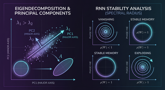
An eigenvector of a matrix A is a vector that doesn't change direction under A's transformation — it only gets scaled. That scale factor is the corresponding eigenvalue: Av = λv. For symmetric matrices (like covariance matrices), all eigenvalues are real. For general square matrices, they may be complex. The set of eigenvalues is the matrix's "spectrum."

In PCA, eigendecomposition of the data's covariance matrix Σ reveals the principal components — the directions of maximum variance. The eigenvectors give you the rotation into the principal component coordinate system, and the eigenvalues tell you how much variance each component explains. This is mathematically identical to SVD of the data matrix (with the singular values related to eigenvalues by σᵢ = √λᵢ for the symmetric case).

For Recurrent Neural Networks, the eigenvalues of the recurrent weight matrix W_h are literally the stability criterion. At each timestep, the hidden state is updated as h_t = tanh(W_h h_{t-1} + ...). If any eigenvalue of W_h has magnitude > 1, the hidden state will grow exponentially — exploding gradients. If all eigenvalues have magnitude < 1, the hidden state contracts toward zero — vanishing gradients, meaning the network forgets everything older than a few steps. This is why gradient clipping and careful initialization of W_h (often to an orthogonal matrix, where all eigenvalues have magnitude exactly 1) is so critical for training RNNs.

⚠️ Spectral Radius Controls RNN Memory

The spectral radius ρ(W_h) = max|λᵢ| determines how long an RNN's memory persists. ρ < 1: exponential forgetting. ρ = 1: stable long-term memory (theoretically). ρ > 1: unstable. LSTMs and GRUs solve this by using gating mechanisms that effectively maintain a spectral radius near 1 adaptively. When you see vanishing gradient problems in RNNs, check the spectral radius of your recurrent weight matrix first — it will almost always be significantly below 1.

---

04Norms, Inner Products, and the Mathematics of Attention

Here's the thing most tutorials miss: the scaled dot-product attention in transformers — softmax(QKᵀ/√d_k)V — is a direct application of inner product geometry. The dot product Qᵢ · Kⱼ measures the cosine similarity between the query and key vectors, scaled by their magnitudes. The √d_k scaling corrects for the fact that in high-dimensional spaces, dot products grow with dimension even for random orthogonal vectors. Without it, the softmax saturates (one key gets all the attention mass) because all scores become large.

The L^p norms are the geometric scaffolding of regularization. The L1 norm (‖w‖₁ = Σ|wᵢ|) induces sparsity because its unit ball is a diamond — gradient descent on L1-regularized objectives tends to hit the corners of the diamond, which correspond to sparse solutions. The L2 norm (‖w‖₂ = √(Σwᵢ²)) penalizes large weights more severely, shrinking all weights proportionally without zeroing them. The L∞ norm (max|wᵢ|) controls the maximum absolute weight. Lasso regression uses L1, Ridge uses L2, and their combination ElasticNet uses both simultaneously.

The Frobenius norm extends L2 to matrices: ‖A‖_F = √(Σᵢⱼ Aᵢⱼ²) = √(trace(AᵀA)) = √(Σσᵢ²). It's the natural "size" metric for weight matrices and the loss function for matrix factorization problems (including the original Netflix Prize recommendation challenge). Critically, the Frobenius norm has a beautiful relationship to SVD: it equals the L2 norm of the singular value vector. This means minimizing weight matrix Frobenius norms during training is equivalent to regularizing the singular values — damping the matrix's "stretching" capability in all directions.

💡 Orthogonality Is the Foundation of Efficient Representations

Orthogonal vectors (inner product = 0) are the most informationally efficient representations — they share no redundancy. This is why PCA outputs are orthogonal (each component captures unique variance), why orthogonal weight initialization works better than random Gaussian initialization for deep networks, and why the attention mechanism's separate Q/K/V projections are designed to learn complementary (ideally orthogonal) subspaces. Anything you can do to push your representations toward orthogonality is likely to improve both training efficiency and representational capacity.

---

05Tensors and Einstein Summation: The Language of Deep Learning

Standard matrix algebra handles 2D arrays. Deep learning routinely operates on 3D, 4D, and higher-dimensional tensors — batched sequences, multi-head attention, 3D convolutional feature maps. The Einstein summation convention (einsum) provides a compact, expressive notation for these operations that maps directly to hardware-efficient implementations.

In einsum notation, each tensor dimension gets a letter. Shared letters are summed over (contracted). Output letters specify which dimensions survive. The attention computation is torch.einsum('bqd,bkd→bqk', Q, K) — batch (b), query position (q), key position (k), model dimension (d). The d dimension is shared between Q and K but absent from the output, so it's summed over: for each (batch, query, key) triple, sum the products of Q[b,q,:] and K[b,k,:] — computing their dot product. This single line of notation replaces batched matrix multiplication that would take several lines to express clearly.

Einsum isn't just notation — it's an optimization target. Both PyTorch and TensorFlow's einsum implementations route to optimized BLAS (Basic Linear Algebra Subprograms) operations under the hood, using hardware-specific optimizations for tensor contractions. The einsum compiler in PyTorch can often find the optimal evaluation order for complex multi-tensor contractions, avoiding materializing large intermediate tensors. This is why reimplementing attention from scratch using explicit loops is dramatically slower than the einsum version — even on CPU.

💡 Einsum Common Patterns in Transformers

Mastering these 5 einsum patterns covers ~90% of transformer implementations: (1) Batch matrix multiply: 'bik,bkj→bij' — the core of attention. (2) Multi-head attention scores: 'bhqd,bhkd→bhqk'. (3) Output projection: 'bhqd,hdo→bqo'. (4) Layer norm: operates on last dim, no einsum needed. (5) Feed-forward: 'bqd,df→bqf'. Once you can write these from scratch, you truly understand the transformer architecture — everything else is engineering details.

attention_einsum.py — attention from scratch

import torch
import torch.nn.functional as F
import math

def multi_head_attention(Q, K, V, mask=None):
 """
 Q, K, V: (batch, heads, seq_len, d_head)
 Returns: (batch, heads, seq_len, d_head)
 """
 d_head = Q.shape[-1]

 # Step 1: Attention scores via scaled dot-product (einsum)
 # 'bhqd,bhkd→bhqk' — for each (batch,head), compute Q·Kᵀ
 scores = torch.einsum('bhqd,bhkd->bhqk', Q, K) / math.sqrt(d_head)

 # Step 2: Optional causal mask (for decoder)
 if mask is not None:
 scores = scores.masked_fill(mask == 0, float('-inf'))

 # Step 3: Softmax over key dimension
 attn_weights = F.softmax(scores, dim=-1)

 # Step 4: Weighted sum of values
 # 'bhqk,bhkd→bhqd' — weight each value by attention score
 output = torch.einsum('bhqk,bhkd->bhqd', attn_weights, V)

 return output, attn_weights # return weights for visualization

# Every einsum subscript tells a geometric story:
# b=batch, h=head, q=query pos, k=key pos, d=dimension
# 'bhqd,bhkd→bhqk': project queries and keys into score space (d contracted)

---

06Jacobian and Hessian: The Calculus That Trains Your Network

Every gradient you compute during backpropagation is a special case of the Jacobian. The Jacobian matrix J of a vector-valued function f: ℝⁿ → ℝᵐ is the m×n matrix of all partial derivatives: Jᵢⱼ = ∂fᵢ/∂xⱼ. Backpropagation computes vector-Jacobian products (VJPs) efficiently using the chain rule — this is what autograd frameworks actually do under the hood when you call loss.backward(). You're not computing full Jacobian matrices (which would be enormous); you're computing the product of the loss gradient with each layer's Jacobian, propagating the gradient signal backward through the computational graph.

The Hessian H is the matrix of second-order partial derivatives: Hᵢⱼ = ∂²L/∂wᵢ∂wⱼ. It describes the curvature of the loss surface — how steeply the gradient itself is changing. Positive definite Hessian means you're in a local minimum (the loss curves up in all directions). Indefinite Hessian (some positive, some negative eigenvalues) means you're at a saddle point. The Hessian is what makes Newton's method (θ = θ − H⁻¹∇L) so much faster than gradient descent — it adjusts step sizes based on local curvature — but computing and inverting the full Hessian for a 175-billion-parameter model is completely infeasible.

Modern adaptive optimizers approximate the Hessian's diagonal. AdaGrad maintains the sum of squared gradients as a diagonal curvature estimate, effectively dividing each parameter's learning rate by the square root of this accumulated curvature. Adam maintains exponentially decaying averages of first and second gradient moments — a more sophisticated diagonal Hessian approximation with memory. This is why Adam converges faster than vanilla SGD on most deep learning problems: it's doing approximate second-order optimization at the cost of storing one extra scalar per parameter.

Jacobian: J[i,j] = ∂f_i/∂x_j
Hessian: H[i,j] = ∂²L/∂w_i∂w_j
Adam update: θ -= α · m̂/(√v̂ + ε) where m̂,v̂ ≈ first/second moments of ∇L ⚠️ Vanishing Gradients Are a Jacobian Product Problem

During backpropagation through L layers, the gradient passes through L Jacobian matrices multiplicatively. If each Jacobian has spectral norm < 1 (which happens with sigmoid activations in the saturated regime, or poor weight initialization), the product of L such matrices can be exponentially small — vanishing gradients. ReLU's Jacobian has eigenvalues exactly 1 for active neurons and 0 for inactive ones, which is why ReLU networks train much better than sigmoid networks. Batch normalization further stabilizes Jacobian norms by keeping pre-activation distributions in the linear region of activation functions.

---

07Low-Rank Approximation: How LLMs Get Smaller

The Eckart-Young theorem is one of the most important results in applied linear algebra: the best rank-k approximation of a matrix A (in Frobenius norm) is obtained by keeping only the top-k singular values in the SVD. This isn't just mathematically elegant — it's the foundation of every matrix compression technique used in modern LLMs.

Imagine you have a 4096×4096 weight matrix in a large transformer — 16 million parameters. If its effective rank is 256, you can approximate it with two matrices: A (4096×256) and B (256×4096), totaling about 2 million parameters — an 8× reduction with minimal accuracy loss. This is what happens in post-training quantization and matrix decomposition: we exploit the observed fact that trained weight matrices in LLMs often have much lower effective rank than their full shape would suggest. The weights have "specialized" into a lower-dimensional structure during training.

LoRA (Low-Rank Adaptation) takes this insight and applies it to fine-tuning: instead of updating the full weight matrix W, keep W frozen and add a low-rank update ΔW = AB where A ∈ ℝ^(d×r), B ∈ ℝ^(r×d), r << d. The hypothesis is that the fine-tuning task can be captured in a low-dimensional subspace even if the full weight matrix has high rank. This hypothesis has been empirically validated across hundreds of fine-tuning experiments — rank 8 or 16 LoRA adapters often achieve 95%+ of full fine-tuning performance at 1% of the parameter cost.

✅ How to Choose LoRA Rank in Practice

The optimal LoRA rank depends on task complexity and base model size. Simple style/format adaptation: rank 4–8 sufficient. Domain-specific knowledge adaptation: rank 16–32. Complex capability addition (new reasoning skills): rank 64–128. A principled approach: perform SVD on the weight updates from a small full fine-tuning run, plot the singular value decay, and choose rank where the cumulative explained variance exceeds 95%. This gives you the task-specific rank before committing to a full LoRA training run.

---

08Cholesky Decomposition and Probabilistic Models

Every positive definite matrix A can be written as A = LLᵀ where L is a lower triangular matrix. This is the Cholesky decomposition — the matrix equivalent of taking a square root. It's roughly twice as fast as LU decomposition and numerically more stable, making it the preferred method for solving linear systems involving positive definite matrices.

In Gaussian Processes, the covariance matrix K of observations is positive definite. Computing predictions requires solving Kα = y for α, which naively requires inverting K — O(n³) in the number of observations. The Cholesky approach: decompose K = LLᵀ, solve two triangular systems (O(n²) each), and reuse the decomposition for prediction variance computation. This is the standard implementation in GPyTorch and other GP libraries. Without Cholesky, GPs would be practical only for very small datasets.

In variational inference for Bayesian neural networks, you often need to parameterize a covariance matrix Σ of the variational posterior. If you parameterize Σ directly, you have to enforce positive definiteness constantly during optimization. The Cholesky trick: parameterize L instead of Σ, and compute Σ = LLᵀ. The only constraint is that L's diagonal elements are positive — enforce this with softplus or exponentiation. This is called the "Cholesky parameterization" of positive definite matrices and appears in normalizing flows, reparameterized variational autoencoders, and structured prediction models.

💡 Cholesky Is Also Used in Sampling from Multivariate Gaussians

To sample x ~ N(μ, Σ), you don't directly sample from the correlated distribution. Instead: (1) decompose Σ = LLᵀ, (2) sample z ~ N(0, I) (independent standard normals), (3) compute x = μ + Lz. This is the reparameterization trick in its most explicit form — the same trick that makes VAEs trainable via backpropagation through the sampling operation. Every time you train a VAE, you're implicitly using Cholesky (with a diagonal covariance, L reduces to a diagonal matrix of standard deviations).

---

synthesisHow the Matrix Connects Everything

Every forward pass of a neural network is a cascade of linear transformations (weight matrices) and nonlinear activations, and every backward pass is a cascade of Jacobian-vector products propagating gradient signals. SVD reveals the structure and effective rank of each transformation. Eigendecomposition governs stability. Norms control regularization. Einstein summation expresses the high-dimensional operations efficiently. The Hessian explains why adaptive optimizers outperform plain gradient descent. Low-rank approximation explains why LLMs can be compressed and fine-tuned efficiently. And Cholesky enables the probabilistic models that give AI systems calibrated uncertainty.

None of these are separate topics — they're the same mathematical objects viewed from different angles. SVD and eigendecomposition are related (SVD is eigendecomposition of AᵀA). Norms connect to singular values (Frobenius = L2 of singular values, spectral norm = largest singular value). The Jacobian IS the weight matrix for a single linear layer. Low-rank approximation IS truncated SVD. Understanding these connections gives you the ability to transfer insights across domains: insights from Gaussian Processes inform attention mechanisms, insights from spectral analysis inform RNN design, insights from matrix compression inform fine-tuning strategy.

---

getting startedYour Linear Algebra Mastery Roadmap

la_mastery_path.py

# Week 1: Foundations — implement these from scratch in NumPy
# - Matrix multiplication, transpose, inverse
# - QR decomposition (Gram-Schmidt)
# - LU decomposition with partial pivoting

# Week 2: Decompositions
import numpy as np
U, S, Vt = np.linalg.svd(A) # SVD
vals, vecs = np.linalg.eig(A) # Eigendecomposition
L = np.linalg.cholesky(A) # Cholesky

# Week 3: Apply to AI
# - Implement PCA using SVD (not sklearn)
# - Implement a recommender system using matrix factorization
# - Analyze spectral radius of an RNN weight matrix
# - Implement scaled dot-product attention with einsum

# Week 4: Advanced
# - Implement a rank-k SVD approximation and measure reconstruction error
# - Compute Jacobian of a neural network layer using torch.autograd
# - Visualize eigenvalue distribution of transformer weight matrices
# - Implement LoRA from scratch and verify it matches the SVD intuition

# Key resources (implement, don't just read):
# - Gilbert Strang "Introduction to Linear Algebra" (Chapter 6-8)
# - 3Blue1Brown Essence of Linear Algebra (visual intuition first)
# - fast.ai Computational Linear Algebra (numerical methods focus)

FAQFrequently Asked Questions

How is SVD used in transformers and LLMs? + SVD is used in transformers in multiple ways. First, LoRA (Low-Rank Adaptation) fine-tuning restricts weight updates to be low-rank matrices A and B, which is mathematically equivalent to saying the weight update's SVD has rank at most r. Second, SVD analysis of trained weight matrices reveals their effective rank and guides compression decisions. Third, some attention mechanisms use low-rank factorizations of the attention score matrix to reduce the O(n²) complexity. Fourth, post-training quantization methods often use SVD to identify the most important singular vectors and preserve them with higher precision. Understanding SVD lets you understand exactly what information is preserved and what is discarded in every compression or efficient attention scheme. What is the Jacobian and why does it matter for backpropagation? + The Jacobian of a function f: ℝⁿ → ℝᵐ is the m×n matrix of all partial derivatives J[i,j] = ∂f_i/∂x_j. In backpropagation, gradients flow backward through each layer. At each layer, the gradient of the loss with respect to the layer's input is computed as the vector-Jacobian product: ∂L/∂x = Jᵀ(∂L/∂y). PyTorch's autograd doesn't compute full Jacobians (which would be huge); it computes these VJPs efficiently using the chain rule. When you add a new custom operation to PyTorch, you implement its backward function by specifying this VJP. The Jacobian is also the foundation for understanding vanishing/exploding gradients: if all layer Jacobians have spectral norm < 1, the product of L Jacobians (and thus the gradient signal) decays exponentially with depth. How do eigenvalues relate to PCA and dimensionality reduction? + PCA computes the eigendecomposition of the data covariance matrix Σ = (1/n)XᵀX (for centered data). The eigenvectors of Σ are the principal components — the directions of maximum variance in the data. The corresponding eigenvalues are the amounts of variance explained by each principal component. To reduce to k dimensions, you keep only the k eigenvectors with the largest eigenvalues. This is equivalent to performing SVD on the data matrix X: the right singular vectors of X are the principal components, and the singular values are √(n × eigenvalues of Σ). The key insight: PCA finds the subspace that preserves the most variance — and the math that defines "most variance" is the eigendecomposition of the covariance matrix. What is the difference between L1 and L2 regularization geometrically? + The geometric difference is in their unit balls (the set of weight vectors with norm ≤ 1). The L2 unit ball is a sphere — smooth, no corners. Gradient descent on L2-regularized objectives slides smoothly toward the origin, shrinking all weights proportionally toward zero but rarely zeroing any weight exactly. The L1 unit ball is a diamond (hypercube in higher dimensions) — with sharp corners at the coordinate axes. Gradient descent on L1-regularized objectives tends to get "stuck" at corners of the diamond, which correspond to sparse solutions where many weights are exactly zero. This is why Lasso (L1) produces sparse models and Ridge (L2) produces small but non-sparse models. For feature selection, L1. For stabilizing training, L2. For both, ElasticNet. Why does the √d_k scaling in attention prevent softmax saturation? + In d_k-dimensional space, two random orthogonal vectors have dot product approximately N(0, d_k) — the variance grows linearly with dimension. Without scaling, for large d_k (e.g., 64), attention scores can be in the range [-100, 100], which causes softmax to become nearly one-hot (almost all attention mass on a single key). This makes gradients vanish: the derivative of softmax is near zero when one element dominates. Dividing by √d_k normalizes the scores to approximately N(0, 1) variance regardless of d_k, keeping softmax in a region with meaningful gradients. This is the linear algebra reason for the √d_k — it's not a heuristic but a direct consequence of the expected variance of high-dimensional dot products. How does Cholesky decomposition enable efficient Gaussian Processes? + A Gaussian Process with n training points requires a covariance matrix K of size n×n. Making predictions requires computing K⁻¹y (the regression weights) and K⁻¹k (for prediction variance). Direct inversion is O(n³) and numerically unstable. Cholesky decomposition factors K = LLᵀ in O(n³) time, but then enables solving K x = b in O(n²) time by forward/backward substitution on the triangular factors. More importantly, the Cholesky factor L can be reused for all subsequent predictions: compute L once, then solve for new test points in O(n²) each. Additionally, log det(K) = 2 Σᵢ log Lᵢᵢ, enabling efficient log-likelihood computation for hyperparameter optimization. Cholesky isn't just faster — it's more numerically stable because positive definite matrices have well-conditioned Cholesky factors even when the matrix itself is ill-conditioned. What is the spectral radius and how does it affect RNN training? + The spectral radius ρ(W) is the largest absolute eigenvalue of a matrix: ρ(W) = max_i |λᵢ|. For RNNs, the spectral radius of the recurrent weight matrix W_h determines how information propagates through time. If ρ(W_h) > 1, applying W_h repeatedly amplifies signals — hidden states and gradients grow exponentially. If ρ(W_h) < 1, repeated application shrinks signals — vanishing gradients. The ideal for long-term memory is ρ = 1, achieved by initializing W_h as an orthogonal matrix. Orthogonal matrices have all eigenvalues on the unit circle |λ| = 1, preserving signal magnitudes perfectly through time. LSTM's forget gate achieves a similar effect adaptively, learning when to "clamp" the effective spectral radius based on context. Echo State Networks take this to an extreme, using a fixed random W_h with ρ slightly below 1 and only training the output layer. Why should I learn einsum notation for deep learning? + Einsum notation offers three concrete advantages over explicit loops or matmul calls. First, expressiveness: complex multi-dimensional operations that would require 3-4 lines of reshape + matmul become a single readable line. Second, performance: torch.einsum and np.einsum route to optimized BLAS implementations for specific contraction patterns, often using hardware acceleration not available via Python loops. Third, debuggability: the string notation makes the shape transformations explicit — you can read exactly which dimensions are contracted and which survive, making shape errors easier to diagnose. For transformer implementations specifically, einsum lets you write the full attention computation in 2-3 lines while making the query/key/value/head dimensions explicitly visible. Every serious ML engineer working with transformers should be fluent in einsum notation.

🔢 Linear Algebra Lab

Four experiments: SVD visualization, eigenvalue stability, attention with einsum, and low-rank compression.

Unit circle → A = UΣVᵀ transformation · blue = input · violet = output

SVD Geometric Visualizer A[0,0] 2.0 A[0,1] 0.5 A[1,0] 0.3 A[1,1] 1.5 — σ₁ (large) — σ₂ (small) — Effective rank — det(A) = σ₁σ₂

Watch how the unit circle (blue) transforms into an ellipse (violet). The singular values σ₁ and σ₂ are the semi-axes of that ellipse.

RNN hidden state over time-steps

RNN Spectral Stability Spectral radius ρ 1.00 Time steps 50 Hidden dimension 4 1.00 Spectral radius — Final ‖h‖ — Stability — Grad ratio (t=50/1)

Attention weight matrix — each row = how a query attends to all keys

Attention Einsum Demo Sequence length 8 Model dim d_k 16 Temperature scale 1/√d_k — Avg attention entropy — Max attention weight einsum: 'bhqd,bhkd→bhqk' scale: / √d_k = / 4.00 softmax over k dimension

Singular value spectrum + rank-k approximation error

SVD Low-Rank Compression Matrix size m×n 64×64 Target rank k 8 True rank of matrix Low (≈20) — Frobenius error % — Variance kept — Param reduction — Compression quality