Inside the Transformer: How GPT Actually Processes Language

How GPT & Transformers Actually Work · 4,100 words · 4 interactive labs · April 2026

Inside the Transformer:
How GPT Actually Processes Language

175 billion parameters. Tokens. Embeddings. Softmax. Attention. The architecture that changed everything in 2017 — demystified from first principles, with interactive experiments you can run right now.

Read the Deep Dive ↓ Open the Lab ⚗️ Table of Contents

1. What GPT Actually Stands For
2. Inside a Transformer: Data Flow
3. The Deep Learning Premise
4. Tokens: Breaking Language Apart
5. Word Embeddings: Meaning as Geometry
6. Unembedding: From Vector to Prediction
7. Softmax & Temperature
8. Getting Started: Build It Yourself

01What GPT Actually Stands For — And Why the Last Letter Is the Only One That Matters

Every week someone types a question into ChatGPT and watches it answer fluently, and most of them have no idea what's actually happening inside. They see a chatbot. What's actually running is a sequence of matrix multiplications so carefully constructed that it can predict the next word in a sentence with uncanny accuracy. To understand why that's not magic, start with the name itself.

G is for Generative — these models produce new text. P is for Pretrained — the model learned from a vast corpus of text before you touched it, and that prefix implies there's room to fine-tune it on specific tasks afterward. But T — Transformer — is the word that matters. A transformer is a specific neural network architecture invented at Google in 2017, and it's the singular invention responsible for the entire current wave of AI capability. Every model you've heard of that produces impressive language output — GPT-3, GPT-4, Claude, Gemini, LLaMA — is a transformer or something derived from one.

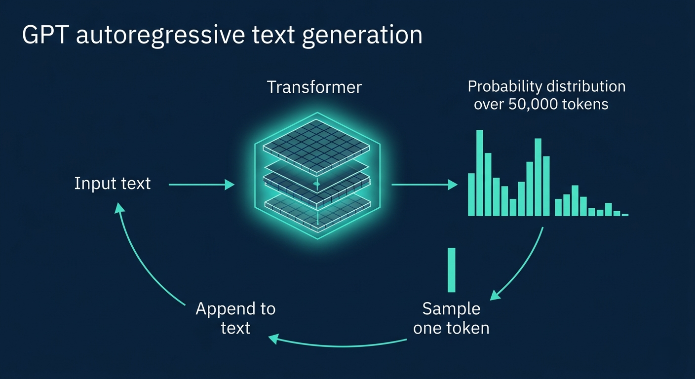
Here's the thing most tutorials miss: the core task of a transformer isn't "being smart" or "understanding language." It's much simpler and much more profound: given a sequence of text, predict a probability distribution over what token might come next. That's it. The intelligence emerges from doing this task at scale, with enough parameters, trained on enough data. The "chatbot" behavior comes from a clever trick of formatting the input as a system prompt + user turn + assistant turn, and then having the model predict what a helpful assistant would say. There's no separate "chat" brain — just a very good next-token predictor applied recursively.

🔮 Myth-Busting: ChatGPT Isn't "Thinking" — It's Sampling

When ChatGPT generates a response, it's not "thinking through" an answer and then typing it. It's sampling tokens one at a time from a probability distribution, appending each one, and re-running the forward pass. The impression of deliberation is an illusion created by the model having learned patterns of deliberative text. Understanding this explains both its strengths (very fast generation) and its failures (confidently wrong "reasoning").

---

02Inside a Transformer: How Data Actually Flows

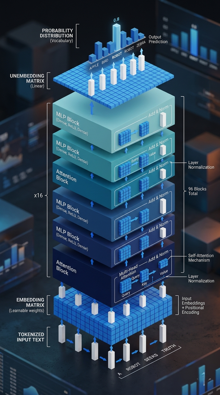
Picture this: you feed the sentence "The cat sat on the" into a transformer. What happens next is a sequence of transformations so elegant it almost seems designed by accident. The text gets broken into tokens. Each token becomes a vector — a list of numbers, 12,288 of them in GPT-3. These vectors flow through alternating blocks of two types: attention blocks and multi-layer perceptron (MLP) blocks. At the end, the very last vector gets multiplied by an unembedding matrix to produce a probability distribution over the next token. The whole thing repeats for every new word.

The attention block is where vectors "talk to each other." The word "model" means something different in "machine learning model" versus "fashion model" — and the attention block is what figures that out, updating each vector's meaning based on the context around it. The MLP block (sometimes called the feed-forward layer) processes each vector independently, in parallel. Think of it as asking a long list of questions about each token and updating it based on the answers. These two blocks alternate, stacking 96 times in GPT-3, each layer refining the representations further.

Everything — every single computation — reduces to matrix-vector multiplication. The 175 billion parameters in GPT-3 live in just under 28,000 matrices, organized into 8 categories. There's a mathematical elegance to this: backpropagation, the training algorithm that adjusts all these weights, requires operations to be differentiable, and matrix multiplication is beautifully differentiable. The choice of this specific structure isn't arbitrary — it's mandated by the mathematics of how you train things at scale.

✅ The Blue/Gray Mental Model

When studying transformer architecture, always separate two kinds of numbers: weights (the model's "brain" — learned during training, fixed during inference) and activations (the data flowing through — changes for every input). Weights are permanent; activations are ephemeral. 175B parameters are all weights. The vectors flowing through the network are activations. Confusing these two is the single most common source of misunderstanding in transformer explanations.

---

03The Deep Learning Premise: Why 175 Billion Knobs Work

Here's a question worth sitting with: why does having 175 billion adjustable numbers produce anything coherent? Why doesn't it just produce noise? The answer lies in understanding what deep learning actually is as a discipline — not as AI hype, but as an engineering paradigm.

Deep learning describes any model that uses the backpropagation training algorithm on a layered, parameterized structure. The key insight is that these models scale remarkably well with both data and compute — a property most earlier ML approaches lack. Linear regression has two parameters and fits a line. A neural network has billions and fits the manifold of human-generated text. The complexity of the parameter space matches the complexity of the task. The simplest version — linear regression — has two parameters (slope, intercept). GPT-3 has 175 billion. But the structure in both cases is the same: tunable numbers that interact with data through weighted sums, trained by minimizing a loss function.

The critical constraint is that everything must be differentiable — which is why you use smooth activation functions (ReLU, GELU) instead of hard decision trees, and why every operation reduces to matrix multiplication. This isn't a stylistic preference; it's a hard requirement of backpropagation. The transformer's architecture choices — attention, MLP layers, residual connections, layer normalization — all exist within this constraint, chosen because they work, not because someone designed them top-down from first principles.

💡 Scaling Laws: The Empirical Foundation

A 2020 paper by Kaplan et al. at OpenAI established that language model performance scales predictably with three factors: model size (parameters), dataset size (tokens), and compute (FLOPs). Crucially, the scaling is smooth and power-law — double the parameters and performance improves by a predictable margin. This "scaling hypothesis" was the bet that OpenAI, Anthropic, DeepMind and others placed enormous resources on. It's why "make it bigger" kept working as a strategy from GPT-1 through GPT-4.

param_count.py

# GPT-3 parameter breakdown — where do 175B come from?

vocab_size = 50_257
embed_dim = 12_288 # d_model
n_layers = 96
n_heads = 96
context_size = 2048

# Embedding matrix W_E
embedding_params = vocab_size * embed_dim # ~617M
# Unembedding matrix W_U (same shape, transposed)
unembedding_params = vocab_size * embed_dim # ~617M

# Per transformer layer: attention + MLP
attn_params_per_layer = 4 * embed_dim * embed_dim # Q,K,V,O projections
mlp_params_per_layer = 8 * embed_dim * embed_dim # 4x expansion, 4x contraction
params_per_layer = attn_params_per_layer + mlp_params_per_layer

total = embedding_params + unembedding_params + n_layers * params_per_layer
print(f"Total parameters: {total/1e9:.1f}B")
# → Total parameters: ~174.6B ✓

---

04Tokens: The Unit of Language in Transformers

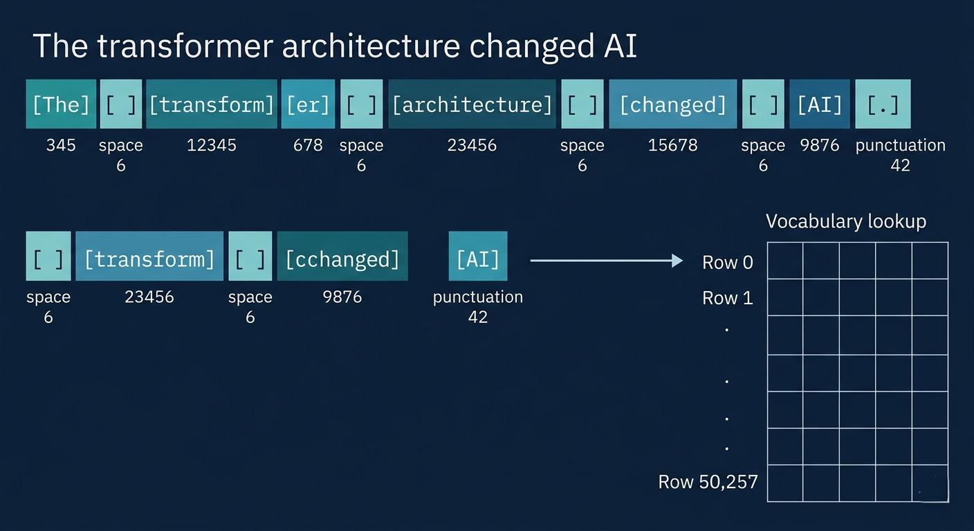
Before any matrix multiplication happens, text has to become numbers. The mechanism that does this is tokenization, and it's subtler than it first appears. You might assume each word becomes one token, but that's not how it works. A transformer has a fixed vocabulary — 50,257 entries in GPT-3 — consisting of not just words, but subword pieces and common character combinations. "unhappy" might tokenize as ["un", "happy"]. "ChatGPT" might become ["Chat", "G", "PT"]. Punctuation, spaces, code syntax — all get their own tokens.

Why subword tokens rather than full words? A full-word vocabulary would need millions of entries to handle the long tail of rare words, technical terms, and neologisms. Character-by-character tokenization would make sequences prohibitively long (more tokens = more computation). Subword tokenization — specifically Byte-Pair Encoding (BPE) in most modern transformers — strikes the balance: common words are single tokens, rare words decompose into recognizable pieces, and the vocabulary stays manageable.

The practical consequence: the context window of a transformer is measured in tokens, not words. GPT-3's 2048-token context corresponds to roughly 1,500 words of English text. This is why early ChatGPT seemed to "forget" early parts of long conversations — once the conversation exceeded the context window, those tokens literally weren't in the input anymore. Modern models have pushed this to 128K tokens (GPT-4 Turbo), 200K (Claude), and even 1M+ for some specialized architectures.

⚠️ Tokens Are Not Words — And This Matters Practically

API pricing for language models is almost always denominated in tokens, not words. English text averages about 1.3 tokens per word, but non-English text, code, and mathematical notation can have much higher token density. Chinese characters often map to 2–3 tokens each. A 1000-word document might be 1,300 English tokens or 2,800 tokens in Japanese. Always tokenize your inputs first when cost-estimating API calls — the difference can be 2–3× for non-Latin scripts.

tokenization.py

import tiktoken # OpenAI's tokenizer library

# Load GPT-3/GPT-4's BPE tokenizer
enc = tiktoken.get_encoding("cl100k_base") # used by GPT-3.5, GPT-4

text = "ChatGPT is a large language model."
tokens = enc.encode(text)
print("Tokens:", tokens)
print("Count:", len(tokens)) # → 8 tokens

# Decode to see the pieces
pieces = [enc.decode([t]) for t in tokens]
print("Pieces:", pieces)
# → ['Chat', 'GPT', ' is', ' a', ' large', ' language', ' model', '.']

# Non-English has higher token density
jp_text = "大規模言語モデル" # "Large language model" in Japanese
jp_tokens = enc.encode(jp_text)
print(f"Japanese: {len(jp_tokens)} tokens for 8 chars") # → 14 tokens!

---

05Word Embeddings: How Meaning Becomes Geometry

Once you have tokens, you need to turn them into numbers that a neural network can process. The mechanism is the embedding matrix — a lookup table with one 12,288-dimensional vector per token in the vocabulary. At initialization, these vectors are random. After training, they've been tuned to represent meaning geometrically: words with similar meanings cluster together in the high-dimensional space, and differences between word vectors encode semantic relationships.

The classic example: take the vector for "king," subtract the vector for "man," add the vector for "woman," and you land near the vector for "queen." The model has apparently learned to encode gender as a direction in this space. More surprising: if you subtract Germany from Italy and add Hitler, you land near Mussolini — the model learned "WWII Axis leader" as a geometric relationship. Perhaps most delightfully: subtract Germany from Japan, add sushi, and you're near bratwurst. These aren't hardcoded — they emerge from training on human-generated text.

Here's the counterintuitive insight: embeddings aren't just static word meanings. In a transformer, the initial embedding is only the starting point. As the vector flows through attention blocks and MLP blocks, it gets updated — pulled and tugged by context. The vector that started as "king" might, by the end of the network, encode "king who lived in Scotland, who usurped the throne, described in Shakespearean English." The embedding dimension needs to be large (12,288 in GPT-3) precisely because it needs room to encode this much contextual nuance.

💡 Dot Products Measure Semantic Similarity

In embedding space, the dot product between two vectors is a direct measure of semantic alignment. Positive dot product: similar meaning. Zero: unrelated. Negative: opposite or contrasting. This is why the attention mechanism (coming in the next chapter) relies so heavily on dot products — it's asking "how related are these two words?" and getting back a scalar that directly encodes the answer. Building intuition for dot products now pays massive dividends when studying attention.

embeddings.py

import gensim.downloader as api
import numpy as np

# Load a word2vec model (smaller than GPT-3 but illustrates the concept)
model = api.load("word2vec-google-news-300")

# Classic analogy: king - man + woman ≈ queen
result = model.most_similar(
 positive=['king', 'woman'],
 negative=['man'], topn=3
)
print("king - man + woman:", result)
# → [('queen', 0.71), ('monarch', 0.62), ('princess', 0.58)]

# Dot product as similarity measure
king_vec = model['king']
queen_vec = model['queen']
noise_vec = model['bicycle']

print(f"king · queen: {np.dot(king_vec, queen_vec):.2f}") # high
print(f"king · bicycle: {np.dot(king_vec, noise_vec):.2f}") # low

---

06Unembedding: Converting the Final Vector Into a Prediction

After the input has passed through 96 alternating attention and MLP blocks, you have a sequence of context-rich vectors — each one having soaked up meaning from the entire surrounding text. The last vector in this sequence now needs to produce an actual prediction: which token comes next? This is the unembedding step, and it's a near-mirror of the embedding step.

The unembedding matrix W_U has one row per token in the vocabulary (50,257 rows), each row as long as the embedding dimension (12,288 entries). Multiply the final context vector by W_U and you get a list of 50,257 raw numbers — one "score" per possible next token. The word Snape gets a high score when the context includes Harry Potter, least favorite teacher, Professor. The word Voldemort might get a slightly lower score. The word bicycle gets a tiny score.

Here's a subtle but important architectural detail: during training, it's more efficient to produce predictions from every vector in the final layer simultaneously — not just the last one. Each position in the sequence predicts what comes after it. This means training on a 2048-token context gives you 2048 training signal examples from a single forward pass — a massive efficiency gain that shapes how the model trains. At inference time (when chatting), you only care about the last position's prediction.

🔥 Weight Tying: The Elegant Trick

In many transformer implementations (including GPT-2 and some GPT-3 variants), the embedding matrix W_E and the unembedding matrix W_U are the same matrix — just transposed. This is called weight tying. The reasoning: if the embedding maps tokens to semantic vectors, the unembedding should do the reverse. Tying the weights enforces this symmetric relationship and cuts ~617M parameters from the model. It's a constraint that turns out to be beneficial — the model can't develop "import embeddings" and "output embeddings" that diverge from each other.

unembedding.py

import torch
import torch.nn as nn

class GPTHead(nn.Module):
 def __init__(self, vocab_size=50257, embed_dim=768):
 super().__init__()
 self.ln_f = nn.LayerNorm(embed_dim)
 self.unembed = nn.Linear(embed_dim, vocab_size, bias=False)

 def forward(self, x):
 # x: (batch, seq_len, embed_dim) — last layer activations
 x = self.ln_f(x) # layer norm
 logits = self.unembed(x) # → (batch, seq_len, vocab_size)
 return logits # raw scores (logits)

# Weight tying: share embedding ↔ unembedding
embed = nn.Embedding(50257, 768)
head = GPTHead()
head.unembed.weight = embed.weight # ← tie the weights
# Now embedding and unembedding share exactly the same parameters

---

07Softmax & Temperature: Turning Raw Scores Into Probability

The unembedding step produces 50,257 raw numbers — logits — that don't sum to 1, include negative values, and have no valid probabilistic interpretation as-is. Softmax is the function that converts them into a proper probability distribution in one elegant step: exponentiate every value (this makes them all positive), then divide each by their sum (this normalizes them to sum to 1). The result: large logits dominate the distribution, small logits get probability close to zero, and negative logits get probability near-zero but never exactly zero.

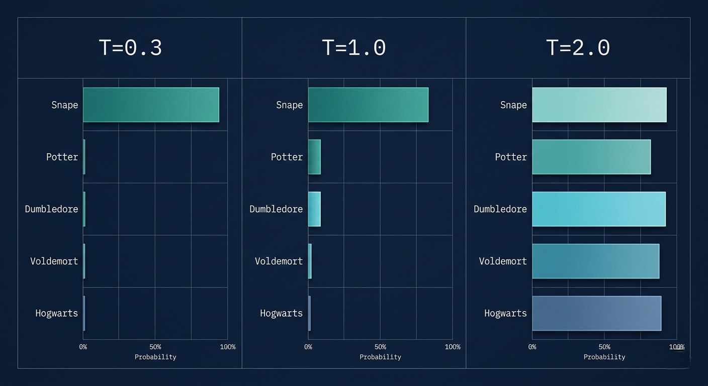
The temperature parameter T is the tunable knob that controls how "confident" the sampling is. Insert T into the exponent denominator: softmax(logits/T). At T=1, standard behavior. At T→0, all probability mass concentrates on the single highest-scoring token — the model always picks the "most likely" next word, resulting in deterministic but often repetitive output. At T=2, the distribution flattens — lower-probability tokens get a real chance to be chosen, introducing creativity and variety at the cost of coherence. The API doesn't allow T>2, which is an arbitrary safety constraint, not a mathematical one.

Understanding temperature gives you a concrete, mechanistic explanation for the "creativity" dial in language model APIs. Higher temperature isn't "more creative" in a human sense — it's just sampling from a flatter distribution, giving unlikely tokens a better shot. Sometimes that produces brilliant unexpected prose; sometimes it produces word salad. The model's capability ceiling doesn't change with temperature — only how conservatively it samples from what it knows.

💡 Logits vs Probabilities — Know the Difference

ML engineers distinguish carefully: logits are the raw, unnormalized scores output by the unembedding matrix. Probabilities are what you get after passing logits through softmax. Cross-entropy loss operates on logits directly (PyTorch's nn.CrossEntropyLoss applies softmax internally). Sampling requires probabilities. Greedy decoding compares logits directly (same result as comparing probabilities). This distinction matters when debugging model outputs — many bugs come from applying softmax twice or forgetting to apply it at all.

softmax_temperature.py

import numpy as np

def softmax_temp(logits, T=1.0):
 """Softmax with temperature control."""
 scaled = logits / T
 exp_x = np.exp(scaled - scaled.max()) # numerical stability
 return exp_x / exp_x.sum()

# Example: 5 candidate next tokens with raw logits
logits = np.array([8.2, 4.1, 2.0, 1.3, -1.5])
words = ['Snape', 'Potter', 'Malfoy', 'Dumbledore', 'bicycle']

for T in [0.3, 1.0, 2.0]:
 probs = softmax_temp(logits, T)
 print(f"\nTemperature T={T}:")
 for w, p in zip(words, probs):
 bar = '█' * int(p * 40)
 print(f" {w:12s} {bar} {p:.3f}")

# T=0.3: Snape ████████████████████████████████████ 0.998 (overconfident)
# T=1.0: Snape ██████████████████████ 0.959
# T=2.0: Snape ████████████ 0.621 (more variety)

---

08Getting Started: Build a Mini-GPT From Scratch

The best way to understand a transformer is to build a tiny one. Andrej Karpathy's nanoGPT is the canonical starting point — a clean implementation of GPT-2 architecture in ~300 lines of PyTorch that trains character-level language models. Below is a self-contained setup to get you running a real transformer on your own text in minutes.

mini_gpt_setup.sh + train.py

# Step 1: Clone and install
git clone https://github.com/karpathy/nanoGPT
cd nanoGPT
pip install torch tiktoken numpy

# Step 2: Prepare training data (Shakespeare example)
python data/shakespeare_char/prepare.py

# Step 3: Train a tiny model (runs on CPU in ~10 minutes)
python train.py config/train_shakespeare_char.py \
 --device=cpu --compile=False \
 --eval_iters=20 --log_interval=10 \
 --block_size=64 --batch_size=12 \
 --n_layer=4 --n_head=4 --n_embd=128 \
 --max_iters=2000 --lr_decay_iters=2000 \
 --dropout=0.0

# Step 4: Sample from your trained model
python sample.py --out_dir=out-shakespeare-char \
 --start="To be or not to be"

embedding_explorer.py

# Explore word embeddings from a trained model
import torch

# Load trained nanoGPT checkpoint
ckpt = torch.load('out/ckpt.pt', map_location='cpu')
embed_matrix = ckpt['model']['transformer.wte.weight'] # W_E

print(f"Embedding matrix shape: {embed_matrix.shape}")
# → torch.Size([65, 128]) (65 chars, 128-dim embedding)

# Find nearest neighbors in embedding space
def nearest_neighbors(token_id, topk=5):
 query = embed_matrix[token_id]
 sims = (embed_matrix @ query) / (
 embed_matrix.norm(dim=1) * query.norm()
 )
 top = sims.topk(topk+1)
 return [(chr(i), f"{s:.3f}") for i, s in
 zip(top.indices[1:].tolist(), top.values[1:].tolist())]

synthesisHow It All Connects

The arc from text to prediction is now clear: tokenize → embed (W_E) → flow through 96 alternating attention and MLP blocks → unembed (W_U) → softmax → sample. The 175 billion weights distributed across 28,000 matrices are all learned through backpropagation on next-token prediction. The training signal is simple: was the actual next token the one with the highest probability? If not, adjust weights to make it higher.

What makes transformers work isn't any single component. It's the combination of: high-dimensional embeddings that can encode rich semantic relationships, attention mechanisms that update those embeddings based on context, deep stacking that allows representations to become progressively more abstract, and scale that allows the model to find patterns humans never explicitly programmed. The next chapter covers attention — the mechanism that does the contextual updating — which is widely considered the heart of the whole architecture.

---

FAQFrequently Asked Questions

What's the difference between GPT-3 and GPT-4? + OpenAI hasn't published GPT-4's architecture details, but the known differences are: GPT-4 is multimodal (accepts images), has a much larger context window (up to 128K tokens), and significantly better reasoning and factual accuracy. Rumored but unconfirmed: GPT-4 is a Mixture of Experts (MoE) architecture — multiple smaller models that specialize, with a routing mechanism deciding which expert handles each token. The total parameter count is unknown. The fundamental transformer architecture described here applies to both, but with significant engineering improvements. Why can't transformers "remember" previous conversations? + Transformers are stateless — they have no persistent memory between calls. Each API call processes the entire conversation history (system prompt + all turns) as a single sequence. Once that sequence exceeds the context window, early tokens are dropped. This is why you can't have a 10,000-message conversation with ChatGPT and expect it to remember message 1 perfectly. Some systems implement external memory retrieval (RAG) or sliding window attention to work around this, but the core architecture is fundamentally a fixed-window function. What is the difference between a language model and a chatbot? + A language model (LLM) is the raw next-token predictor. A chatbot is an LLM that's been fine-tuned with Reinforcement Learning from Human Feedback (RLHF) or similar techniques to behave helpfully and follow instructions, and wrapped with a system prompt that establishes the chat format. ChatGPT started as GPT-3.5, then was RLHF-fine-tuned to produce InstructGPT/ChatGPT. The underlying model is the same architecture; the difference is in the training and prompting. What is a "context window" and why does size matter? + The context window is the maximum number of tokens a transformer can process in a single forward pass. It limits how much text the model can "see" at once. For GPT-3, that was 2,048 tokens (~1,500 words). For Claude 3, it's 200,000 tokens (~150,000 words — roughly 500 pages). Larger context windows enable: summarizing entire books, processing long codebases, maintaining multi-hour conversations. The computational cost of attention scales quadratically with context length (O(n²)), which is why large context windows are technically challenging. Modern techniques like Flash Attention and grouped-query attention help manage this cost. What exactly is a "logit" in the context of language models? + In machine learning, a logit is the raw, unnormalized output of a classification head before any probability function is applied. In a language model, the logits are the 50,257 raw scores produced by multiplying the final context vector by the unembedding matrix W_U. They can be any real number — positive, negative, or zero. After applying softmax, they become probabilities that sum to 1. The word "logit" comes from statistics (log-odds), but in ML it's used loosely to mean "pre-softmax scores." You'll hear ML engineers say "the logit for the word 'cat'" — they mean the raw score for that token before normalization. How does a transformer handle images and audio, not just text? + The same architecture works for any modality as long as you can represent the input as a sequence of vectors. For images: divide the image into fixed-size patches (e.g., 16×16 pixels), flatten each patch into a vector, embed it. This is Vision Transformer (ViT). For audio: convert to a spectrogram and break it into time-frequency patches. For video: patch across both space and time. The transformer itself doesn't know or care whether the vectors came from text, images, or audio — it just processes sequences of vectors. This generality is part of why transformers have become the universal backbone for modern AI. Is temperature the same as "creativity" in language models? + Not quite, though they're correlated. Temperature controls how much probability is spread across lower-ranked tokens during sampling. Higher temperature → more uniform distribution → lower-probability tokens can be chosen → output feels more varied and "creative." But "creativity" in a human sense involves generating genuinely novel ideas, not just picking less expected words. A high-temperature model might produce unexpected word choices while still being factually wrong or incoherent. Real creativity in LLMs — generating new analogies, reasoning novel solutions — emerges from the model's learned representations, not temperature. Temperature is a sampling parameter, not an intelligence parameter. What comes after attention blocks — what do MLP layers actually do? + Attention blocks update token representations based on context (which other tokens are relevant). MLP blocks update each token independently, without looking at neighbors. A useful framing: attention handles "who relates to whom"; MLP handles "given what this token now means, what do I know about it?" Research suggests MLP layers act as key-value memories — specific input patterns ("the Eiffel Tower is in...") activate specific neurons that store facts. The MLP layers are responsible for much of the factual knowledge stored in the model, while attention handles compositional and contextual reasoning. This is explored in detail in the next chapter.

⚗️ Transformer Lab

Four experiments to build intuition about tokenization, embeddings, softmax temperature, and architecture scale — all in your browser.

Input Text Token Visualization Click a token to inspect its ID → Tokenization Stats 0 Tokens 0 Characters — Chars/Token — % of GPT-3 ctx Token ID Histogram Interesting Tokenizations Hello world! ChatGPT sentence Japanese text Python code

Note: This uses a simplified BPE simulation. For exact OpenAI tokenization, use tiktoken in Python.

2D projection of 3D embedding space slice · Hover for word · Click to select

Embedding Explorer Vector Components (12D preview) Nearest Neighbors Analogy Arithmetic king − man + woman = ? (click Find Analogy) 12288 Dimensions 50,257 Vocab Size 617M Parameters — Dot Product

Probability distribution over top-10 candidate tokens

Softmax curve shape at different temperatures

Temperature & Sampling Controls Temperature T 1.00 Context: Harry Potter Sampling Mode — Sampled Token — Probability — Entropy (bits) — Perplexity

Architecture diagram — scale with slider to see how GPT sizes compare

Architecture Parameters Embedding Dimension d_model 768 Number of Layers 12 Number of Heads 12 Vocab Size 50,257 Context Length 2048 — Total Params — Embed Params — Attn Params — MLP Params Compare: GPT-2 has 1.5B params (d=1600, L=48). GPT-3 has 175B (d=12288, L=96). nanoGPT: ~10M (d=384, L=6). Drag sliders to understand what drives parameter count.