Backpropagation Explained: The Algorithm That Teaches Neural Networks

Backpropagation Deep Dive · 3,800 words · 4 interactive experiments · April 2026

Backpropagation Explained:
The Algorithm That Teaches Neural Networks

Every time a neural network gets a little better, backpropagation is working behind the scenes. Here's exactly what it does — not the formula soup, but the real mechanical intuition — plus four labs where you can feel every piece of it working.

Read the Deep Dive ↓ Open the Lab ⚗️ Table of Contents

1. What Backpropagation Actually Is
2. The Single Training Example Walkthrough
3. Three Avenues to Nudge a Neuron
4. Hebbian Theory & "Wiring Together"
5. Propagating Backwards Through Layers
6. Stochastic Gradient Descent
7. The Dirty Secret: Data Hunger
8. Getting Started: Code It Yourself

01What Backpropagation Actually Is

Imagine you're a coach watching a team play their first game. They lose, badly. Now you have to figure out: which players made the biggest mistakes? Who needs the most coaching? You can't just yell "everyone was wrong" and expect improvement. You need to trace the loss back to specific decisions, rank them by impact, and give proportional feedback to each player. That's backpropagation — except the players are weights and biases, the game is a training example, and "coaching" means computing a precise gradient.

Backpropagation is the algorithm that computes the gradient of the cost function with respect to every single weight and bias in the network. That gradient — a 13,000-dimensional vector in our digit-recognition example — tells each parameter exactly how much it contributed to the current error, and in which direction it should change to reduce that error. Without backpropagation, computing this gradient would be computationally intractable. With it, the computation is elegant and efficient.

Here's the thing most tutorials miss: backpropagation isn't a learning algorithm itself — it's a gradient-computation algorithm. The actual learning happens via gradient descent, which uses backprop's output to update weights. Backprop just answers the question: "how sensitive is the cost to each weight right now?" The answer to that question, computed for every weight simultaneously, is what makes neural network training possible at scale.

🔮 Myth-Busting: "Backprop Teaches the Network"

Backpropagation doesn't "teach" anything. It computes. The gradient it produces tells you which direction to nudge weights to decrease cost on the current training example. The actual adjustment is made by gradient descent. Think of backprop as a very smart accountant who calculates where money was lost — and gradient descent as the manager who makes the financial decisions based on that report.

what_backprop_returns.py

import torch
import torch.nn as nn

model = nn.Sequential(nn.Flatten(), nn.Linear(784,16), nn.ReLU(),
 nn.Linear(16,16), nn.ReLU(), nn.Linear(16,10))

X, y = next(iter(train_loader))
loss = nn.CrossEntropyLoss()(model(X), y)

# This one line IS backpropagation
loss.backward()

# Inspect what backprop computed for each layer
for name, p in model.named_parameters():
 if p.grad is not None:
 print(f"{name:22s} | grad shape: {str(p.grad.shape):18s} | norm: {p.grad.norm().item():.5f}")

# Output:
# 1.weight | grad shape: torch.Size([16,784]) | norm: 0.04231
# 1.bias | grad shape: torch.Size([16]) | norm: 0.00891
# 3.weight | grad shape: torch.Size([16,16]) | norm: 0.12044
# 5.weight | grad shape: torch.Size([10,16]) | norm: 0.28812 ← largest near output

---

02The Single Training Example Walkthrough

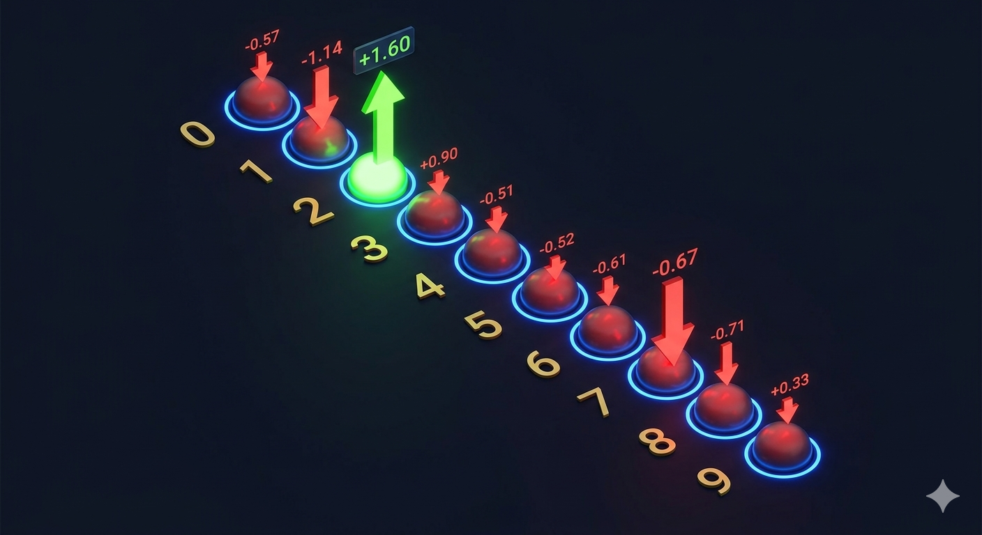
Let's make this concrete. Take a single training image — a handwritten 2. The network hasn't been trained yet, so its output layer is a mess: something like [0.5, 0.8, 0.2, 0.6, 0.1, 0.4, 0.3, 0.7, 0.2, 0.1]. The correct output should be [0, 0, 1, 0, 0, 0, 0, 0, 0, 0]. Looking at that gap, the network's job description becomes very specific: nudge the "2" neuron's activation up, nudge everything else down.

But here's the critical nuance that gradient descent cares about: the nudges should be proportional to how far off each output is from its target. The "1" neuron showing 0.8 (should be 0) needs a bigger downward nudge than the "8" neuron showing 0.2 (should be 0) — it's already much closer to zero. This proportionality isn't arbitrary; it directly follows from the derivative of the squared-error cost function. Larger errors produce larger gradients, producing larger weight updates, which is exactly what you want.

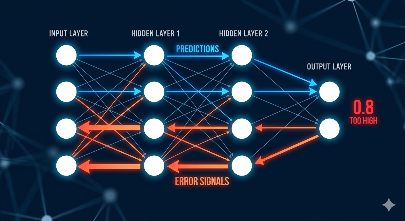
Picture this from the network's perspective. We're not changing activations directly — we can only touch weights and biases. So the output layer's "wishlist" (nudge digit-2 up, everything else down) gets translated into: how do I change the weights and biases that produced this output to move it closer to what we wanted? That translation is the first backward pass. And then, crucially, the same logic applies one layer earlier: how do the activations of the second-to-last hidden layer need to change? And the layer before that? All the way to the input.

💡 Why "Proportional to the Error" Matters

Using squared error (MSE) instead of absolute error gives you this proportionality for free. The derivative of (output − target)² is 2(output − target) — which is largest when the error is largest. This means the gradient automatically focuses correction energy on the worst-performing outputs. It's not a choice someone made arbitrarily; it's a mathematically elegant consequence of the cost function's shape.

output_nudges.py

import numpy as np

 # Network output for an image of "2"
 output = np.array([0.5, 0.8, 0.2, 0.6, 0.1, 0.4, 0.3, 0.7, 0.2, 0.1])
 target = np.array([0, 0, 1, 0, 0, 0, 0, 0, 0, 0])

 # The "wishlist" — proportional to error
 nudges = 2 * (output - target) # derivative of MSE

 for i, n in enumerate(nudges):
 direction = "▲ nudge UP " if n < 0 else "▼ nudge DOWN"
 print(f"Digit {i}: {direction} | magnitude: {abs(n):.2f}")

 # Digit 0: ▼ nudge DOWN | magnitude: 1.00
 # Digit 1: ▼ nudge DOWN | magnitude: 1.60 ← largest, most wrong
 # Digit 2: ▲ nudge UP | magnitude: 1.60 ← needs most increase
 # Digit 3: ▼ nudge DOWN | magnitude: 1.20
 # ...
 # Digit 8: ▼ nudge DOWN | magnitude: 0.40 ← already close to 0

---

03Three Avenues to Nudge a Single Neuron

Zoom in on a single output neuron — the one for digit 2 — whose activation we want to increase. Its activation is computed as a weighted sum of all 16 neurons in the previous layer, plus a bias, all passed through an activation function. That gives us exactly three distinct levers to pull: change the weights, change the bias, and (indirectly) change the previous layer's activations.

The weight lever is the most interesting. Not all weights are equally powerful here. A weight connecting to a highly-active neuron in the previous layer has more influence than a weight connecting to a dim neuron — because activation is multiplied by the weight, a large activation amplifies the effect of even a small weight change. This means backpropagation naturally prioritizes changing weights that connect strongly-firing neurons to neurons we want to change. This is a subtle but crucial point: the gradient isn't just about direction, it's about leverage.

The bias lever is simpler — you just add or subtract from the weighted sum regardless of what the previous layer is doing. But the previous-layer activation lever is the most recursive and fascinating. We can't change those activations directly (they're determined by even earlier weights and biases), but we can note what we wish they were. If a previous-layer neuron connects to digit-2 with a positive weight, we want that neuron to be more active. If it connects with a negative weight, we want it dimmer. This "wish list" for the previous layer is exactly the error signal that gets propagated backward — hence backpropagation.

✅ The Three Levers — Ranked by Impact

When backprop adjusts a weight, the magnitude of the adjustment depends on two things simultaneously: how large the error in the downstream neuron is, and how active the upstream neuron is. This multiplicative relationship means:

• High error × high activation → largest weight update (most bang for buck)
• High error × low activation → moderate weight update
• Low error × high activation → moderate weight update
• Low error × low activation → tiny weight update (this connection barely matters right now)

three_avenues.py

# Simplified manual backprop for one output neuron
# Shows the three adjustment channels

def backprop_one_neuron(output_act, target, prev_activations, weights, bias, lr=0.1):
 # Error signal (∂Loss/∂output) for MSE loss
 error = 2 * (output_act - target)

 # Avenue 1: Adjust bias — independent of previous layer
 new_bias = bias - lr * error

 # Avenue 2: Adjust weights — scaled by prev layer activation
 # Bigger prev activation → bigger weight change → more influence
 new_weights = [w - lr * error * a
 for w, a in zip(weights, prev_activations)]

 # Avenue 3: Desired change in previous layer activations
 # Positive weight → want prev neuron brighter; negative → dimmer
 desired_prev_changes = [-error * w for w in weights]
 # (can't apply directly — propagate these desires further back)

 return new_weights, new_bias, desired_prev_changes

---

04Hebbian Theory: Neurons That Fire Together, Wire Together

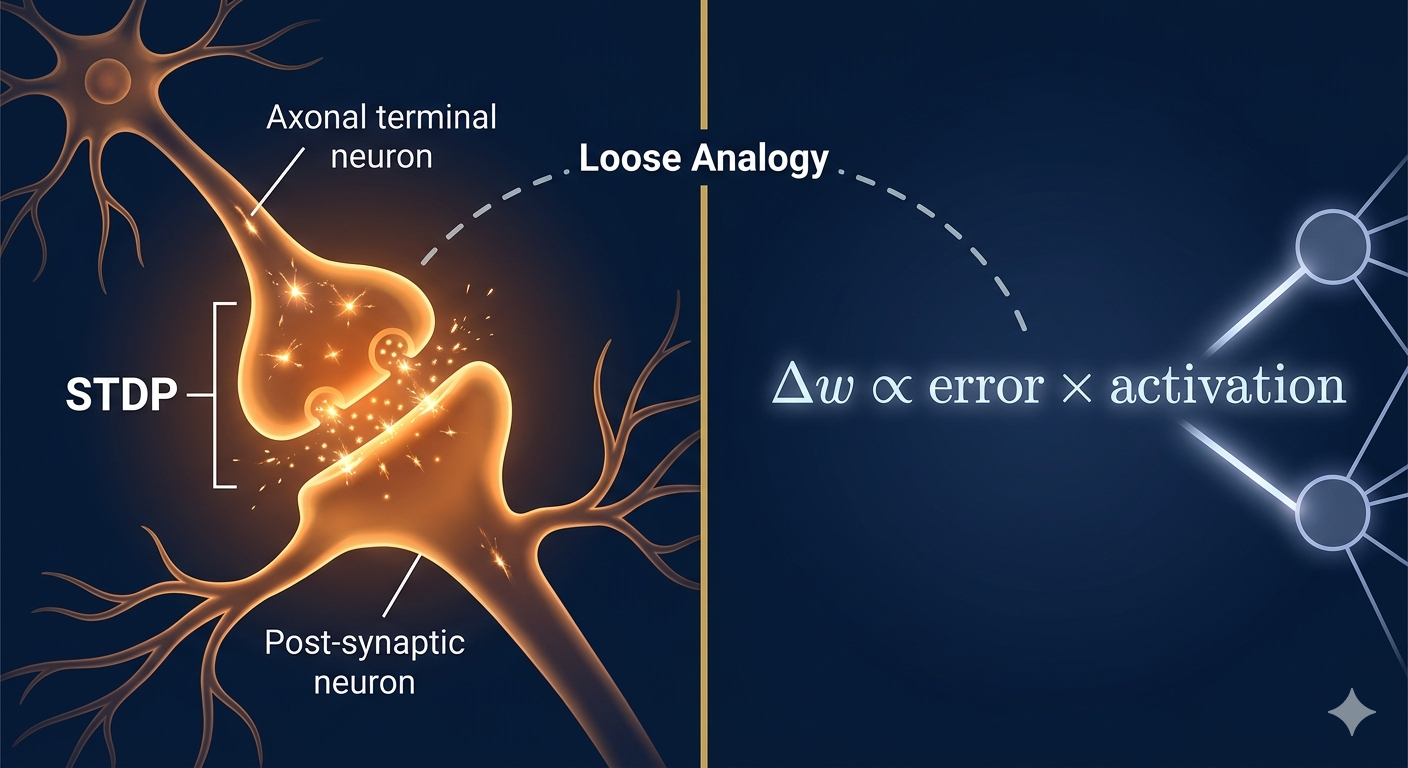
There's a fascinating parallel between backpropagation's weight update rule and a 70-year-old theory in neuroscience. Donald Hebb proposed in 1949 that synaptic connections between neurons strengthen when both neurons fire simultaneously. "Neurons that fire together, wire together" — the slogan that has outlasted entire fields of neuroscience research.

Look at backpropagation's weight update for a moment: the change to a weight is proportional to both the error signal and the activation of the upstream neuron. If a neuron is active (firing) while we're trying to make the downstream neuron more active (fire), its connection gets strengthened. If the downstream neuron shouldn't be firing (incorrect classification), connections from active upstream neurons get weakened. The math mirrors Hebb's theory strikingly closely, even though one emerged from neuroscience and the other from applied mathematics decades later.

Here's the important asterisk though: the analogy breaks down quickly under scrutiny. Biological Hebbian learning is local — each synapse only needs information about the two neurons it connects. Backpropagation is explicitly non-local — it requires propagating error signals from the output all the way back through the entire network. Real brains don't have a supervisor providing the correct output. Backpropagation does. This difference is significant, and the question of how biological brains actually learn remains one of neuroscience's great open problems. The convergence between the two is poetic, but not deep.

⚠️ Don't Over-Read the Biological Analogy

Backpropagation works because it correctly implements the chain rule of calculus — not because it mimics the brain. The biological parallel is a fun observation, not a design principle. Real neural learning in the brain is thought to involve mechanisms like spike-timing-dependent plasticity (STDP), neuromodulators, and local credit assignment — none of which map cleanly onto backprop. Knowing the difference matters if you're studying either field seriously.

---

05Propagating Backwards: How Credit Flows Through Layers

So we've established what the output layer wants from the second-to-last hidden layer. But each hidden neuron is being pulled in different directions by different output neurons simultaneously. The digit-2 neuron wants certain hidden neurons to be brighter, while the digit-7 neuron wants some of those same neurons to be dimmer (since they shouldn't fire for a 7). Backpropagation resolves this conflict by adding together all these competing desires, weighted by how strongly each output neuron cares about each hidden neuron.

Once you have the net desired change for the second-to-last layer, the process repeats recursively. That layer now has its own "wishlist" for the layer before it, computed in exactly the same way: multiply by connection weights, sum across all connections. This recursive application of the same logic — from output backward through every layer to the input — is why the algorithm is called backpropagation. The error signal literally propagates backward through the computation graph.

The computational efficiency comes from the chain rule: instead of computing each weight's gradient independently (which would require a separate forward pass per weight — millions of forward passes), backpropagation computes all gradients in a single backward pass. Forward pass: one computation. Backward pass: one more computation. Total work: two passes through the network, regardless of how many weights you have. This is the algorithmic miracle that makes deep learning tractable.

🔥 The Chain Rule — Why Backprop Is O(N) Not O(N²)

If you computed each weight's gradient via finite differences (nudge one weight, see how cost changes), you'd need one forward pass per weight. For 13,000 weights, that's 13,000 forward passes per training step. Backpropagation exploits the chain rule to share intermediate computations — you compute every gradient in a single backward pass. This isn't just faster, it's the difference between feasible (O(N)) and impossible (O(N²)) for large networks.

manual_backprop.py

import numpy as np

class ManualNetwork:
 def __init__(self, sizes):
 self.W = [np.random.randn(j,i) * np.sqrt(2/i)
 for i, j in zip(sizes[:-1], sizes[1:])]
 self.b = [np.zeros((j,1)) for j in sizes[1:]]

 def forward(self, x):
 self.acts = [x] # store all activations for backprop
 self.zs = []
 for W, b in zip(self.W, self.b):
 z = W @ self.acts[-1] + b
 self.zs.append(z)
 self.acts.append(np.maximum(0, z)) # ReLU
 return self.acts[-1]

 def backward(self, y_true, lr=0.01):
 # Start from output error
 delta = 2 * (self.acts[-1] - y_true) # ∂MSE/∂output

 # Propagate backward through each layer
 for l in range(len(self.W)-1, -1, -1):
 # ReLU derivative: 1 if z > 0, else 0
 relu_grad = (self.zs[l] > 0).astype(float)
 delta *= relu_grad

 # Weight gradient: error × upstream activation (Hebbian!)
 dW = delta @ self.acts[l].T
 db = delta

 # Pass error to previous layer (propagate backward)
 if l > 0:
 delta = self.W[l].T @ delta # ← the backward pass

 # Update weights and biases
 self.W[l] -= lr * dW
 self.b[l] -= lr * db

---

06Stochastic Gradient Descent: The Drunk Man Walking Downhill

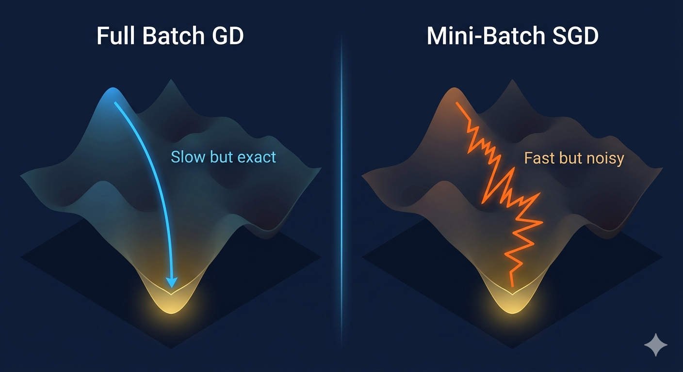
In a perfect world, you'd run backpropagation over all 60,000 training examples, average the gradients, and take one precisely-calculated step downhill. This is called full-batch gradient descent, and it has a beautiful mathematical property: you're always moving in the true direction of steepest descent. It also has a practical problem: it's brutally slow. For 60,000 examples and 13,000 weights, that's a staggering amount of computation per step.

The practical solution — mini-batch stochastic gradient descent — is both pragmatically brilliant and theoretically interesting. RandoDLy shuffle your training data and split it into mini-batches of, say, 32 or 64 examples. Run backpropagation on each mini-batch, average those gradients, take a step. The gradient you compute isn't the true gradient — it's a noisy approximation. But it's a good approximation, and you compute it 937 times faster (60,000 ÷ 64).

Here's the counterintuitive part: the noise isn't just a necessary evil. Research suggests it's actually beneficial. A noisy gradient can kick you out of sharp, narrow minima that have high test error (they don't generalize well) and tends to find flatter, wider minima that generalize better. The "drunk man stumbling down a hill" doesn't find the deepest valley — but the deepest valley might actually be a trap. The flat meadow nearby might generalize better. This is why SGD often outperforms full-batch gradient descent on test performance, even though it's less precise per step.

✅ Choosing Mini-Batch Size: Practical Rules

Mini-batch size is a hyperparameter with real performance implications:

• Batch size 1 (true SGD): Maximum noise, maximum regularization effect, very slow convergence. Rarely used in practice.
• Batch size 32–64: Classic sweet spot. Good GPU utilization, good gradient estimates, good generalization.
• Batch size 256–2048: Better hardware utilization, but may require learning rate scaling (linear scaling rule: lr × (new_batch / old_batch)). Watch for generalization degradation.
• Very large batches (>4096): Can hurt generalization significantly. Use warm-up learning rate schedules and layer normalization to compensate.

sgd_loop.py

import torch
from torch.utils.data import DataLoader

# Mini-batch SGD — the workhorse of deep learning
loader = DataLoader(train_set, batch_size=64, shuffle=True)
# shuffle=True ensures random mini-batches every epoch

for epoch in range(num_epochs):
 for batch_idx, (X, y) in enumerate(loader):
 # Forward pass
 pred = model(X)
 loss = loss_fn(pred, y)

 # Backpropagation — compute gradients over mini-batch
 optimizer.zero_grad() # clear previous gradients
 loss.backward() # backprop over this mini-batch
 optimizer.step() # gradient descent step

 if batch_idx % 200 == 0:
 print(f"Epoch {epoch} | Batch {batch_idx}/{len(loader)}"
 f" | Loss: {loss.item():.4f}")
# One full pass through 60,000 examples = 937 mini-batches of 64

---

07The Dirty Secret: Data Hunger

No algorithm section on backpropagation is complete without confronting the thing that limits it in real practice: backprop is only as good as the data you feed it. The algorithm is mathematically elegant and computationally efficient — but it's trying to minimize a cost function defined over your training set. If your training set doesn't represent the real world well, you're optimizing for the wrong thing.

MNIST feels easy precisely because it's a clean, human-labeled dataset of 70,000 examples. In real DL projects, gathering labeled data is often the hardest part of the entire pipeline — not the modeling, not the training, not the evaluation. Labeling medical images requires radiologists. Labeling legal documents requires lawyers. Labeling speech requires transcriptionists. The cost is real, the time is real, and the quality matters enormously. Backprop will faithfully minimize loss on whatever labels you give it — including wrong ones.

The practical implication: before you worry about architecture choices, activation functions, or learning rate schedules, worry about your data quality. More high-quality labeled examples consistently outperform clever modeling tricks on limited data. This is the uncomfortable truth of applied machine learning that academic papers rarely emphasize. The three highest-leverage investments in any DL project are: data, data, and data. Backpropagation is a tool that amplifies the quality of your data — it can't manufacture signal that isn't there.

🔮 Counterintuitive Insight: More Data > Better Algorithms

A seminal 2001 paper by Banko and Brill showed that across several NLP tasks, increasing training data by 10× consistently outperformed switching to a better algorithm on a smaller dataset. This pattern has held remarkably well across two decades of ML research. Spending 2 weeks collecting better training data will usually beat spending 2 weeks tuning your model architecture — every time. The best model trained on bad data is worse than a mediocre model on excellent data.

---

08Getting Started: Implement Backprop From Scratch

The most powerful way to truly understand backpropagation is to implement it without an autograd library. Here's a complete, working implementation for the MNIST digit network — no PyTorch, no TensorFlow, just NumPy and the chain rule.

backprop_from_scratch.py

import numpy as np
from torchvision import datasets, transforms

# Load and prep MNIST
def load_mnist():
 ds = datasets.MNIST('.', download=True, transform=transforms.ToTensor())
 X = ds.data.numpy().reshape(-1, 784) / 255.0
 y = ds.targets.numpy()
 y_oh = np.eye(10)[y] # one-hot encode
 return X, y_oh

# Network: 784 → 64 → 32 → 10
def init_params():
 return {
 'W1': np.random.randn(784,64) * np.sqrt(2/784),
 'b1': np.zeros(64),
 'W2': np.random.randn(64,32) * np.sqrt(2/64),
 'b2': np.zeros(32),
 'W3': np.random.randn(32,10) * np.sqrt(2/32),
 'b3': np.zeros(10),
 }

def relu(z): return np.maximum(0, z)
def relu_d(z): return (z > 0).astype(float)
def softmax(z): e = np.exp(z - z.max(axis=1, keepdims=True)); return e/e.sum(axis=1, keepdims=True)

def forward_and_backward(X, y, p, lr=0.01):
 N = X.shape[0] # batch size

 # FORWARD PASS
 z1 = X @ p['W1'] + p['b1']; a1 = relu(z1)
 z2 = a1 @ p['W2'] + p['b2']; a2 = relu(z2)
 z3 = a2 @ p['W3'] + p['b3']; a3 = softmax(z3)
 loss = -(y * np.log(a3 + 1e-9)).mean()

 # BACKWARD PASS — chain rule, layer by layer
 d3 = (a3 - y) / N # ∂L/∂z3 (softmax+CE combined)
 p['W3'] -= lr * a2.T @ d3 # weight: error × upstream act
 p['b3'] -= lr * d3.sum(axis=0)

 d2 = (d3 @ p['W3'].T) * relu_d(z2) # propagate backward
 p['W2'] -= lr * a1.T @ d2
 p['b2'] -= lr * d2.sum(axis=0)

 d1 = (d2 @ p['W2'].T) * relu_d(z1) # propagate backward again
 p['W1'] -= lr * X.T @ d1
 p['b1'] -= lr * d1.sum(axis=0)

 return loss

This 40-line implementation contains every concept from this post: the forward pass storing activations, the error computed at the output, the chain-rule multiplication of ReLU derivatives, the weight gradient as error × upstream activation, and the recursive error propagation backward through each layer. Every line maps to something you now understand.

synthesisHow It All Connects

The full three-video arc comes into focus: a neural network is a parameterized function (Part 1). The cost function measures how wrong it is, and gradient descent minimizes that cost (Part 2). Backpropagation efficiently computes the gradient that gradient descent needs (Part 3). Together, these three ideas — differentiable functions, gradient-based optimization, and the chain rule — underpin virtually all of modern deep learning.

What makes backpropagation genuinely elegant is that it doesn't require understanding the entire network at once. Each layer only needs to know two things: the error signal coming from the layer above it, and the activations of the layer below it. Everything else falls out of the chain rule naturally. The global problem of "how should 13,000 weights change?" decomposes into a clean sequence of local computations — which is exactly what makes it implementable, differentiable, and scalable.

---

FAQFrequently Asked Questions

Is backpropagation the same as the chain rule? + Almost, but not quite. Backpropagation is an algorithm that efficiently applies the chain rule to compute gradients in neural networks. The chain rule is the mathematical foundation; backpropagation is the computational implementation that exploits the layered structure of neural networks to share intermediate computations. Without the chain rule, backpropagation wouldn't work. Without backpropagation's efficient implementation, the chain rule applied naively to 13,000 parameters would be computationally prohibitive. Why do we store activations during the forward pass? + Because the backward pass needs them. The weight gradient for any layer is error_signal × upstream_activation. During the forward pass, we compute and store all intermediate activations (a₁, a₂, etc.). During the backward pass, we use these stored activations to compute weight gradients. Without storing them, we'd have to recompute the entire forward pass at each layer of backprop — doubling the computation. This is the memory/compute tradeoff: backprop uses more memory to avoid redundant computation. Gradient checkpointing is a technique that trades back some of this compute to reduce memory usage in very large models. What happens if the activation function isn't differentiable? + ReLU is technically non-differentiable at exactly x=0 (it has a kink there). In practice, this almost never matters — the probability of a neuron's weighted sum being exactly zero is essentially nil. By convention, we define the derivative at 0 as either 0 or 1, and training proceeds without issues. For truly non-differentiable operations, straight-through estimators (STE) allow gradients to "pass through" non-differentiable functions by using an approximate gradient for the backward pass. This is used extensively in quantization and binary neural networks. What is the difference between a gradient and a partial derivative? + A partial derivative measures how the function changes when you change one input while holding all others fixed: ∂L/∂w₁₂₃ for a specific weight. A gradient is the vector of all partial derivatives collected together: ∇L = [∂L/∂w₁, ∂L/∂w₂, ..., ∂L/∂w₁₃₀₀₀]. Backpropagation computes all these partial derivatives simultaneously — one full backward pass gives you the entire gradient vector. Gradient descent then uses this vector to take a step: w ← w − lr × ∇L. Why does zero_grad() need to be called before each backward pass? + PyTorch accumulates (adds) gradients by default — it doesn't overwrite them. If you call loss.backward() twice without zeroing gradients, the second backward pass adds to the first pass's gradients, effectively doubling them. This is intentional design (it's useful for gradient accumulation over multiple mini-batches to simulate larger batch sizes), but for normal training loops you always want fresh gradients per step. Forgetting optimizer.zero_grad() is one of the most common bugs in PyTorch code — and it's insidious because training still proceeds, just with wrong gradient magnitudes. What is gradient accumulation and when should I use it? + Gradient accumulation simulates a larger batch size when you can't fit one in GPU memory. Instead of calling optimizer.step() every batch, you accumulate gradients over N batches (skipping zero_grad), then step once. This is mathematically equivalent to training with batch_size × N, without the memory requirement. Use it when: your GPU can't hold your desired batch size, you're fine-tuning large language models, or you want to train with batch sizes larger than your hardware supports. It adds latency (more forward passes before each update) but enables training configurations otherwise impossible. Can backpropagation fail? What causes it to break down? + Yes, in several ways. Vanishing gradients: error signals shrink exponentially as they propagate backward through many layers, causing early layers to stop learning (common with sigmoid/tanh, fixed by ReLU and residual connections). Exploding gradients: error signals grow exponentially, causing weight updates to be catastrophically large (fixed by gradient clipping or careful initialization). Dead neurons: ReLU neurons that always output zero have zero gradient — they never recover (use Leaky ReLU or careful initialization). Numerical instability: very large or small values cause NaN/Inf (fixed by batch normalization and careful loss function choices). How does automatic differentiation (autograd) relate to backpropagation? + Backpropagation is the algorithm; autograd is the software system that implements it. PyTorch's autograd builds a dynamic computation graph during the forward pass — every operation records which inputs it consumed and how to compute its gradient. When you call .backward(), autograd traverses this graph in reverse, applying the chain rule at each node. This means you can use any Python control flow (if statements, loops, recursion) and autograd handles backpropagation correctly through all of it — because the graph is built dynamically based on the actual execution, not a static description.

⚗️ Backprop Lab

Four hands-on experiments. Feel credit assignment, watch error propagate backward, compare SGD noise, and see gradient magnitude decay across layers.

Orange arrows = backward error signal · Thickness = gradient magnitude · Click a neuron to inspect

Credit Assignment Controls Target Digit 2 Output Noise Level 0.30 Signal Amplification 1.0× Output Layer Errors Layer Gradient Magnitudes 0 Prop Steps — Max Gradient — Min Gradient — Decay Ratio

Try: Change the target digit and watch where error is highest. Increase noise to see more dramatic credit assignment. Notice how gradient magnitude decreases as you go further from the output.

Loss trajectory · Blue=full batch · Orange=mini-batch SGD

Gradient direction field at each step

SGD Configuration Batch Size 64 Learning Rate 0.050 Epochs to Simulate 50 0 Steps — Final Loss — Gradient Noise — Converged? Draw a Digit Backprop State ? Prediction — Loss — Confidence 0 BP Steps Output Probabilities Gradient Magnitudes by Layer Hidden Size 16

Gradient norm per layer across training steps — vanishing gradient visualization

Weight update magnitude heatmap — which weights are being adjusted most?

Gradient Flow Configuration Network Depth 4 Activation Fn Weight Init Scale 1.0× — Max Layer Norm — Min Layer Norm — Vanish Ratio — Gradient Health