Advanced RAG: Stop Hallucinations with Reranking, Hybrid Search & Query Rewriting

Advanced RAG · Production AI · 2026 · 4,000 words · 4 interactive labs · April 2026

Advanced RAG:
Stop Hallucinations with
Reranking, Hybrid Search
& Query Rewriting

Your RAG pipeline works in demos. Users send the exact same phrasing you tested with and it retrieves the right chunks. Then it ships to production. Users phrase things differently. They're vaguer. They use synonyms. They ask multi-hop questions. Your vector search returns tangentially related chunks, the LLM fills the gaps with confident invention, and suddenly your AI product is spreading misinformation about your own product. Here's how to fix it — systematically.

Read the Deep Dive ↓ Open RAG Lab 🧠 Query Rewriting→ Hybrid BM25+Vector→ Cross-Encoder Reranking→ Parent-Child Chunking→ Context Assembly→ LLM Generation Table of Contents

1. Pre-Retrieval: Query Rewriting & Expansion
2. Hybrid Search: BM25 + Dense Vectors
3. Parent-Child Chunking Strategies
4. Cross-Encoder Reranking
5. Context Window Optimization
6. GraphRAG: Knowledge Graphs + RAG

01Pre-Retrieval Optimization: Fix the Query Before It Hits the Index

The naive RAG assumption is that users ask good questions. They don't. Real users ask "what about the pricing thing?" after a 10-turn conversation. They ask "how do I fix this error?" without pasting the error. They ask one question when they actually need the answer to three connected sub-questions. If you feed these queries directly to your vector index, you get back chunks that match the surface-level words rather than the underlying intent — and the LLM, receiving poor context, confidently hallucinates the rest.

Query rewriting solves the first problem: it uses an LLM to rephrase the user's query into a cleaner, more explicit version before retrieval. "What about the pricing thing?" becomes "What is the pricing structure for the Enterprise tier?" This costs one small LLM call upfront but dramatically improves retrieval precision. Query expansion goes further: it generates multiple related queries from the original — synonyms, related concepts, different phrasings — and retrieves for all of them. The union of results covers more of the relevant semantic space. Multi-query generation decomposes complex questions into sub-questions: "Compare the performance and cost of GPT-4o vs Claude Sonnet for document analysis" becomes three separate retrieval queries, each targeting one dimension of the comparison. The results are merged and deduplicated before reranking.

Here's the counterintuitive insight about query rewriting: it's not just about improving queries from naive users. Even well-phrased technical queries benefit from expansion because embedding models have blind spots. Your documentation uses the term "inverted index" but your user asks about "keyword search internals." These are semantically close but not always close enough in embedding space to reliably retrieve the same chunks. Generating synonymous rephrasings before retrieval closes this gap without any changes to your index or embedding model.

💡 HyDE: Hypothetical Document Embeddings

Here's the thing most RAG tutorials miss entirely: Hypothetical Document Embeddings (HyDE) is one of the most powerful pre-retrieval techniques. Instead of embedding the query and searching for similar documents, you ask the LLM to generate a hypothetical answer to the question (even if it hallucinates details), then embed that answer and search for similar documents. The logic: a hypothetical answer looks like a document from your corpus — same vocabulary, same structure — making it a better embedding for retrieval than a short question. HyDE consistently outperforms direct query embedding for complex technical questions. The downside: one extra LLM call per query.

pre_retrieval.py — query rewriting + multi-query

from anthropic import Anthropic
from typing import List

client = Anthropic()

def rewrite_query(original_query: str, conversation_history: str = "") -> str:
 """Rewrite vague or context-dependent queries into standalone questions."""
 prompt = ff"""Given this conversation history:
{conversation_history}

The user asked: "{original_query}"

Rewrite this into a clear, standalone, self-contained question that:
1. Doesn't rely on conversation context
2. Uses precise terminology
3. Specifies what type of answer is needed

Return ONLY the rewritten question, nothing else."""
 response = client.messages.create(
 model="claude-sonnet-4-20250514", max_tokens=200,
 messages=[{"role": "user", "content": prompt}]
 )
 return response.content[0].text.strip()

def generate_multi_queries(query: str, n: int = 3) -> List[str]:
 """Generate N diverse phrasings of the same query for retrieval coverage."""
 prompt = ff"""Generate {n} different search queries that would retrieve 
documents answering: "{query}"

Each query should emphasize different aspects or use different terminology.
Return one query per line, nothing else."""
 response = client.messages.create(
 model="claude-sonnet-4-20250514", max_tokens=300,
 messages=[{"role": "user", "content": prompt}]
 )
 queries = response.content[0].text.strip().split('\n')
 return [query] + [q.strip() for q in queries if q.strip()]

# Usage: retrieve for all queries, deduplicate by doc ID
def multi_query_retrieve(query: str, retriever, k: int = 5) -> list:
 queries = generate_multi_queries(query)
 seen_ids, results = set(), []
 for q in queries:
 for doc in retriever.retrieve(q, k=k):
 if doc.id not in seen_ids:
 seen_ids.add(doc.id); results.append(doc)
 return results

---

02Hybrid Search: When Semantic Isn't Enough

Dense vector search is powerful, but it has a well-known failure mode: exact keyword matching. If a user searches for "RFC 7231 status codes" or "kubectl get pods --namespace kube-system error CrashLoopBackOff", pure semantic search often returns tangentially related documents instead of the exact documentation the user needs. Embedding models encode general semantics; they don't inherently privilege exact string matches. BM25 — the algorithm powering Elasticsearch and Solr for decades — excels at exactly this: term frequency, inverse document frequency, and exact token matching.

Hybrid search combines both worlds: dense vector retrieval (captures meaning, synonyms, paraphrases) and sparse BM25 retrieval (captures exact terms, acronyms, product names, version numbers, error codes). The standard fusion technique is Reciprocal Rank Fusion (RRF): instead of combining raw scores (which have incompatible scales), combine rank positions. If a document ranks 2nd in vector search and 8th in BM25, its RRF score is 1/(k+2) + 1/(k+8) where k is typically 60. RRF is robust to score scale differences and consistently outperforms weighted linear combinations that require tuning.

The practical architecture: run both retrievals in parallel (async), collect top 50 results from each, fuse with RRF, and pass the top 20 fused results to your reranker. The added latency from BM25 is minimal if run concurrently. Vector databases like Qdrant, Weaviate, and Elasticsearch all support hybrid search natively. For Qdrant specifically, sparse vectors (SPLADE or BM25-style) can live alongside dense vectors in the same collection, making hybrid retrieval a single API call.

✅ Use SPLADE Instead of Raw BM25 for Better Sparse Retrieval

Traditional BM25 only sees exact token matches — it can't expand "car" to "automobile" or "vehicle." SPLADE (SParse Lexical AnD Expansion) is a learned sparse retrieval model that produces sparse vectors with vocabulary expansion built in. It retains BM25's exact-match strengths while adding the ability to expand queries and documents with related terms. SPLADE sparse vectors integrate directly with vector databases that support sparse vector fields. For most RAG applications, SPLADE + dense vector hybrid outperforms BM25 + dense vector hybrid by 5-15% on technical retrieval benchmarks. The downside: SPLADE requires generating sparse vectors at index time, adding ~50ms per document during ingestion.

hybrid_search.py — RRF fusion with Qdrant

from qdrant_client import QdrantClient, models
from sentence_transformers import SentenceTransformer

client = QdrantClient("http://localhost:6333")
dense_model = SentenceTransformer('all-MiniLM-L6-v2')

def hybrid_search(query: str, k: int = 20) -> list:
 dense_vec = dense_model.encode(query, normalize_embeddings=True)
 
 results = client.query_points(
 collection_name="docs",
 prefetch=[
 # Dense vector search (semantic meaning)
 models.Prefetch(query=dense_vec.tolist(), using="dense", limit=50),
 # Sparse vector search (exact keyword matching via SPLADE)
 models.Prefetch(query=sparse_encode(query), using="sparse", limit=50),
 ],
 # Reciprocal Rank Fusion — no score calibration needed
 query=models.FusionQuery(fusion=models.Fusion.RRF),
 limit=k,
 # Optional: filter before vector search for metadata constraints
 query_filter=models.Filter(must=[
 models.FieldCondition(
 key="doc_type", match=models.MatchValue(value="technical")
 )
 ])
 )
 return results.points

# RRF formula for manual implementation:
# rrf_score(d) = Σ 1/(k + rank_i(d)) for each ranking i
# k=60 by default, ranks are 1-indexed

---

03Parent-Child Chunking: Retrieve Small, Return Large

Chunking strategy is where most RAG systems quietly fail without anyone realizing it. The naive approach — split every 512 tokens, index those chunks, retrieve those chunks, feed those chunks to the LLM — creates a precision-recall tension. Small chunks (128 tokens) give precise retrieval (the embedding represents one focused concept) but poor context (the LLM receives a fragment without surrounding explanation). Large chunks (1024 tokens) give rich context but poor precision (the embedding is diluted by multiple concepts, making similarity search unreliable).

Parent-child chunking resolves this tension directly: embed small child chunks for retrieval (128 tokens, each representing one focused concept), but return the full parent chunk (512 tokens, the complete section) as context to the LLM. When a child chunk is retrieved, the system fetches its parent automatically. The LLM receives rich, coherent context; the embedding model operates on focused, precise representations. This is the architecture behind LlamaIndex's "Small-to-Big Retrieval" and LangChain's "ParentDocumentRetriever."

Picture this: you're indexing a technical manual. Chapter 3 covers "Authentication." Section 3.2 is "API Key Management." Paragraph 3.2.1 explains "How to rotate API keys." With naive chunking, a query about key rotation might retrieve a 512-token chunk that includes adjacent content about key creation and key deletion — diluting the relevant content with noise. With parent-child chunking, the child chunk is just the 128-token paragraph about key rotation (precise retrieval), but the parent chunk returned to the LLM is the full 512-token section about API Key Management (complete context). Best of both worlds.

🔬 Sentence Window Retrieval: A Simpler Alternative

Parent-child chunking requires storing two representations per document section. A simpler alternative is sentence window retrieval: embed individual sentences for precise retrieval, but return a window of N surrounding sentences (typically 3-5 on each side) as context. This requires only one set of embeddings and stores the window context in the document metadata. Sentence window retrieval is easier to implement but gives less structured context than true parent-child chunking — you return whatever surrounds the matched sentence, which may span paragraph boundaries. For prose documents (articles, documentation), sentence window works well. For structured documents (API references, technical specifications), parent-child respects the natural hierarchy better.

parent_child_chunking.py — implementation

from dataclasses import dataclass, field
from typing import List

@dataclass
class Document:
 parent_id: str
 child_id: str
 parent_text: str # returned to LLM (large, coherent context)
 child_text: str # embedded for retrieval (small, focused)
 metadata: dict = field(default_factory=dict)

def create_parent_child_chunks(text: str, parent_size: int = 512,
 child_size: int = 128, overlap: int = 20) -> List[Document]:
 docs = []
 # Split into parent chunks first
 parent_chunks = split_text(text, chunk_size=parent_size, overlap=50)
 
 for p_idx, parent_text in enumerate(parent_chunks):
 parent_id = ff"parent_{p_idx}"
 # Split each parent into smaller child chunks
 child_chunks = split_text(parent_text, chunk_size=child_size, overlap=overlap)
 
 for c_idx, child_text in enumerate(child_chunks):
 docs.append(Document(
 parent_id=parent_id,
 child_id=ff"{parent_id}_child_{c_idx}",
 parent_text=parent_text, # stored in metadata, returned at query time
 child_text=child_text, # embedded and indexed
 ))
 return docs

# At retrieval time: retrieve by child embedding, return parent text
def retrieve_with_parent_context(query: str, vector_db, embed_model) -> list:
 query_vec = embed_model.encode(query)
 child_results = vector_db.search(query_vec, k=10)
 
 # Deduplicate by parent_id — multiple children may share a parent
 seen_parents = set()
 context_chunks = []
 for result in child_results:
 parent_id = result.metadata['parent_id']
 if parent_id not in seen_parents:
 seen_parents.add(parent_id)
 context_chunks.append(result.metadata['parent_text'])
 return context_chunks # rich context for LLM, precise retrieval

---

04Cross-Encoder Reranking: The Precision Layer

Your hybrid search retrieved 50 candidate documents. Some are highly relevant. Some are tangentially related. Some share vocabulary with the query but answer a completely different question. The vector and BM25 scores tell you how similar the documents are to the query in isolation — but not how well they actually answer it. A cross-encoder reranker solves this by looking at the query and document together, attending to both simultaneously, producing a relevance score that's dramatically more accurate than either dense or sparse retrieval alone.

Unlike bi-encoder models (which embed query and document independently and compare in a shared space), cross-encoders input the query and document concatenated into a single sequence and output a single relevance score. This joint attention is expensive — you can't pre-compute document embeddings, so you must run inference at query time for every (query, document) pair. That's why reranking is a second-pass operation on a small candidate set (50-100 results) rather than a first-pass operation on the full corpus (millions of documents). The latency trade-off is 50-200ms for the reranking pass, but the precision improvement is significant — typically 15-30% improvement in NDCG@10 on technical retrieval benchmarks.

The most widely used rerankers are Cohere Rerank (API-based, simple to integrate, excellent quality), BGE-Reranker (open-source, self-hostable, strong performance), and mxbai-rerank (newer, competitive with Cohere at lower cost). The choice depends on your latency budget, cost model, and data privacy requirements. For sensitive enterprise data, self-hosted BGE-Reranker is the pragmatic choice. For teams prioritizing developer velocity and quality, Cohere Rerank's API with its straightforward SDK is hard to beat.

⚡ Rerank the Right Number of Candidates

Reranking quality depends on the candidate set size. Too few candidates (10): the reranker can only improve ordering within a limited set — if the truly relevant document wasn't in the top 10, reranking can't help. Too many candidates (200): latency grows linearly with candidate count, and most candidates are irrelevant noise. The sweet spot for most production systems: retrieve 50-100 candidates via hybrid search, rerank all of them, return top 5-10 to the LLM. This gives the reranker enough candidates to find the truly relevant documents while keeping reranking latency under 200ms. Always measure your recall@50 (how often is the answer in your top 50 retrieved candidates) before optimizing reranking — if recall@50 is 60%, no amount of reranking will fix the 40% of queries where the answer was never retrieved at all.

reranking.py — cross-encoder pipeline

from sentence_transformers import CrossEncoder
import cohere
from typing import List, Tuple

# Option 1: Self-hosted BGE-Reranker (free, private)
cross_encoder = CrossEncoder('BAAI/bge-reranker-v2-m3')

def rerank_bge(query: str, documents: List[str], top_k: int = 10) -> List[Tuple[int, float]]:
 pairs = [(query, doc) for doc in documents]
 scores = cross_encoder.predict(pairs) # joint attention on all pairs
 ranked = sorted(enumerate(scores), key=lambda x: x[1], reverse=True)
 return [(idx, float(score)) for idx, score in ranked[:top_k]]

# Option 2: Cohere Rerank API (hosted, simple)
co = cohere.Client(api_key="your-api-key")

def rerank_cohere(query: str, documents: List[str], top_k: int = 10) -> list:
 response = co.rerank.create(
 query=query,
 documents=documents,
 model="rerank-v3.5",
 top_n=top_k,
 return_documents=True
 )
 return [
 {"text": r.document.text, "score": r.relevance_score, "index": r.index}
 for r in response.results
 ]

# Full pipeline: retrieve → rerank → assemble context for LLM
def advanced_rag_pipeline(query: str) -> str:
 candidates = hybrid_search(query, k=50) # step 1: hybrid retrieval
 doc_texts = [c.payload['text'] for c in candidates]
 reranked = rerank_bge(query, doc_texts, top_k=8) # step 2: cross-encoder
 context = "\n\n---\n\n".join([doc_texts[i] for i, _ in reranked])
 return call_llm(query, context) # step 3: LLM with good context

---

05Context Window Optimization: What You Put In Is What You Get Out

Modern LLMs have large context windows — 128K, 200K, even 1M tokens. The temptation is to stuff as much retrieved content as possible and let the LLM sort it out. This is a mistake, and it's a surprisingly well-documented one. The "lost in the middle" problem is empirically real: when relevant information is placed in the middle of a long context, LLMs reliably attend less to it than information placed at the beginning or end. Liu et al. (2023) showed this clearly — model performance on multi-document question answering degrades significantly as the position of the relevant document moves toward the middle of the context window.

Context window optimization means being intentional about what you include, how much you include, and where you place it. The most actionable rules: place the most relevant chunks first and last (exploit the primacy and recency effects). Limit context to 3-8 chunks of 512 tokens each — more is rarely better after reranking has done its job. Deduplicate chunks before assembling context; multiple retrieved chunks from the same parent document create redundancy that wastes tokens and dilutes attention. Include a "context preamble" that tells the LLM what type of documents it's receiving and what the query is — this primes attention on the right signals.

💡 Use Contextual Compression Before Sending to LLM

Even well-ranked chunks contain irrelevant sentences. Contextual compression — running each retrieved chunk through an LLM extraction step ("given this question: X, extract only the relevant sentences from this document") — can reduce token count by 40-70% while retaining all relevant information. This is LangChain's ContextualCompressionRetriever pattern. The trade-off: an extra LLM call per chunk. For applications where context window cost and hallucination reduction are top priorities, contextual compression often pays for itself in reduced generation costs and improved accuracy. Skip it when you have high query volume and low latency budget.

---

06GraphRAG: When Vector Search Misses the Relationships

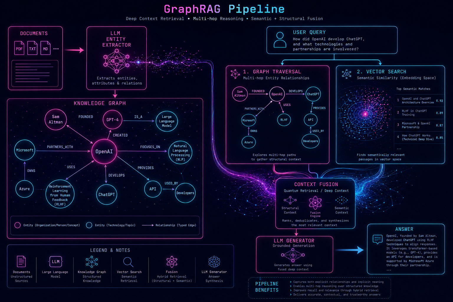
Vector search finds semantically similar chunks. It doesn't know that "BRCA1 gene" relates to "breast cancer risk" which relates to "PARP inhibitor treatment" which relates to "olaparib" — unless those explicit relationships appear in the same chunk. For questions that require multi-hop reasoning across entities and their relationships, pure vector RAG consistently fails. GraphRAG combines a knowledge graph (capturing structured entity-relationship data) with vector retrieval (capturing semantic similarity) to answer questions that neither can handle alone.

Microsoft's GraphRAG framework (2024) formalizes this approach: it first runs an LLM over all documents to extract entities and relationships, builds a knowledge graph, and then at query time uses both graph traversal (who is connected to whom? how?) and vector search (which chunks are semantically relevant?) to assemble context. The result: answers to complex multi-hop questions like "What drugs have been shown effective against conditions involving the same pathway as BRCA1 mutations?" — questions where the answer requires traversing multiple entity relationships that no single chunk contains.

The implementation trade-off is significant: GraphRAG requires an ingestion pipeline that runs LLM inference over your entire corpus to extract entities, which can be expensive for large document sets. It's not the right tool for every use case. GraphRAG shines for knowledge-intensive domains with rich entity relationships: biomedical research, legal case law, financial relationships between entities, and complex technical documentation with extensive cross-references. For general-purpose QA over homogeneous documents (customer support, HR policies, standard documentation), advanced RAG with hybrid search and reranking will outperform GraphRAG at far lower cost.

⚠️ GraphRAG's Cost Can Be Prohibitive at Scale

Microsoft's GraphRAG benchmark paper reported ingestion costs of ~$10 per million tokens for entity extraction. For a 1TB corpus, this is potentially hundreds of thousands of dollars in LLM API costs before you've answered a single query. Mitigations: use smaller, cheaper models (Haiku, Flash) for entity extraction — they're less accurate but dramatically cheaper. Run entity extraction incrementally as new documents are ingested. Use LightRAG (a lighter-weight alternative) which achieves comparable performance with lower extraction overhead. Or use GraphRAG only for your highest-value, most relationship-dense document collections and vanilla Advanced RAG for the rest.

---

synthesisThe Production Advanced RAG Stack

A production advanced RAG pipeline looks like this: incoming query → query rewriting (clarify vague or context-dependent queries) → multi-query generation (3-5 diverse phrasings) → parallel hybrid retrieval for each query (dense vector + SPLADE sparse, fused with RRF) → candidate deduplication → cross-encoder reranking on top 50-100 candidates → parent-child context expansion (retrieve child, return parent) → contextual compression (extract only relevant sentences) → context assembly with primacy/recency optimization → LLM generation with well-crafted system prompt.

Each layer adds latency: ~200ms for multi-query LLM call, ~100ms for parallel hybrid retrieval, ~150ms for cross-encoder reranking, ~200ms for contextual compression. Total added latency versus naive RAG: 500-700ms. Whether that's acceptable depends on your application. For an asynchronous research assistant, yes. For a real-time chat interface, you need to be selective — skip multi-query and contextual compression, keep hybrid search and reranking, which get you 80% of the quality improvement at 30% of the latency cost.

---

FAQFrequently Asked Questions

What is Advanced RAG and how is it different from naive RAG? + Naive RAG: embed the user's query, find the most similar document chunks, concatenate them, send to LLM, get answer. Works in demos, fails in production. Advanced RAG adds layers before and after retrieval to improve precision and recall. Pre-retrieval: query rewriting (clarify vague queries), query expansion (generate synonyms and rephrasings), multi-query generation (decompose complex questions), and HyDE (generate hypothetical answers to embed instead of questions). Post-retrieval: cross-encoder reranking (re-score candidates with a model that sees query + document jointly), contextual compression (extract only relevant sentences), and context assembly optimization. The architectural changes: hybrid BM25+vector retrieval, parent-child chunking, and semantic caching all fall under advanced RAG. The combined effect: dramatically reduced hallucinations and higher answer quality for real-world user queries. What is cross-encoder reranking and why is it better than vector search alone? + Vector search uses bi-encoder models: query and document are embedded independently and compared by cosine similarity. Fast, scalable, but the comparison is limited by what can be encoded into a fixed-size vector. Cross-encoder reranking takes the query and document together, concatenates them into one input sequence, and runs transformer attention over the combined text. This joint attention allows the model to catch subtle query-document relationships that bi-encoders miss: negations, conditional relevance, specific entity matching, and nuanced relevance that requires reading both texts together. The trade-off: cross-encoders can't pre-compute document embeddings, so they run at query time — making them 100-200× slower per document than vector search. This is why reranking is always a second-pass operation on a small candidate set (50-100 docs) after fast vector/hybrid retrieval narrows the field. What is hybrid search in RAG and when should I use it? + Hybrid search combines dense vector retrieval (semantic similarity via embeddings) with sparse keyword retrieval (exact term matching via BM25 or SPLADE). Use it whenever: users query with exact terms, product names, error codes, acronyms, version numbers, or technical jargon. Dense vector search captures conceptual similarity but can miss exact terminology. BM25 excels at exact token matching but misses paraphrases. Reciprocal Rank Fusion (RRF) blends both rankings without needing score calibration. In practice, hybrid search improves recall@10 by 15-25% over pure vector search for technical documentation. Most modern vector databases (Qdrant, Weaviate, Elasticsearch) support hybrid search natively. The only case where you might skip hybrid search: purely conversational QA where users always phrase questions in natural language without technical terms — though even then, hybrid rarely hurts. What is parent-child chunking and how does it improve RAG? + Parent-child chunking resolves the precision-recall tension in RAG chunking. Small chunks (128 tokens) produce precise embeddings (focused on one concept) but give the LLM insufficient context. Large chunks (1024 tokens) give rich context but produce diluted embeddings that match too broadly. The solution: index small child chunks for retrieval (precise matching), but at retrieval time, return the full parent chunk to the LLM (rich context). Multiple child chunks from the same parent automatically deduplicate — you don't send the same parent twice. Implementation: split documents into parent chunks (512 tokens), split each parent into child chunks (128 tokens), store parent text in child chunk metadata, embed child chunks for the vector index. At query time: retrieve by child embedding, fetch parent text from metadata, deduplicate by parent ID, return parent texts as context. What is query rewriting in RAG and when does it help? + Query rewriting uses an LLM to transform a user's query into a better retrieval query before hitting the vector index. It's most valuable for: (1) Conversational context — queries like "what about the second point?" need conversation history resolved into "what is [specific topic] mentioned earlier?" (2) Vague queries — "how do I fix it?" becomes "how do I resolve the authentication error in JWT token validation?" (3) Vocabulary mismatch — user says "make the text bigger" but docs say "increase font size" — rewriting bridges the gap. Query rewriting adds ~200ms latency (one small LLM call) and typically improves retrieval precision by 10-20% for conversational applications. Skip it for: high-volume, low-latency search applications where queries are already well-formed, or when you have tight latency budgets. What is GraphRAG and when should I use it over standard RAG? + GraphRAG combines a knowledge graph (entities and their relationships extracted by an LLM from your documents) with vector retrieval. Use it when: your questions require multi-hop reasoning across entities ("which drugs treat conditions involving the same pathway as gene X?"), your domain has rich entity-relationship structure (biomedical, legal, financial), or when standard RAG consistently fails on questions that span multiple documents. Don't use GraphRAG when: your corpus is large and homogeneous (costs too much to extract entities), your questions are factual lookups from single documents, or you have tight latency requirements (graph traversal adds complexity). Microsoft's GraphRAG framework and LightRAG are the two main open-source implementations. GraphRAG's ingestion cost (LLM over full corpus for entity extraction) can be prohibitive at scale — benchmark carefully before committing. How do I evaluate if my Advanced RAG pipeline is actually better? + RAG evaluation requires measuring both retrieval quality and generation quality separately. For retrieval: measure Recall@K (what fraction of the time is the relevant document in your top K results?), Precision@K (of your top K, how many are actually relevant?), and MRR (Mean Reciprocal Rank — how highly ranked is the first relevant result?). For generation: measure answer faithfulness (does the answer stay grounded in the context? — use an LLM to check), answer relevance (does it answer the actual question?), and context precision (was the retrieved context actually used?). Tools: RAGAS (open-source framework specifically for RAG evaluation), LangSmith (LangChain's observability platform), and custom LLM-as-judge pipelines. The key: build an evaluation dataset of 100-500 (question, expected answer, relevant document) triples from your actual domain before building anything — otherwise you're optimizing blindly. What is Reciprocal Rank Fusion (RRF) in hybrid search? + Reciprocal Rank Fusion (RRF) is the standard algorithm for combining ranked lists from multiple retrieval systems (e.g., vector search and BM25). For each document, RRF computes: score(d) = Σ 1/(k + rank_i(d)) where k is a smoothing constant (typically 60) and rank_i is the document's rank in each list. A document ranked 1st in vector search and 10th in BM25 gets: 1/(60+1) + 1/(60+10) = 0.0164 + 0.0143 = 0.0307. RRF's key advantage over score fusion (weighted combination of raw scores) is robustness: dense vector scores and BM25 scores are on incompatible scales, and calibrating them correctly requires extensive tuning. RRF only uses rank positions, making it scale-invariant and requiring no calibration. It consistently matches or outperforms tuned score fusion in benchmarks, making it the practical default for hybrid search fusion.

🧠 Advanced RAG Lab

Four experiments: query rewriter, hybrid search fusion, reranking demo, and context assembler.

Query Rewriting Simulator Original query (try vague ones) Conversation context (optional) Technique Query Rewriting Transformed Queries — Queries generated — Expected recall lift

RRF fusion — how vector and BM25 rankings combine into final score

Hybrid Search RRF Simulator Documents to rank 8 RRF k constant 60 — Top doc after RRF — Rank changes

Before vs after cross-encoder reranking — relevance score comparison

Cross-Encoder Reranking Demo

Simulate how reranking re-orders vector search results by true relevance.

Candidate pool size 20 Top-K to return 5 — Precision@5 before — Precision@5 after — Improvement ~150ms Rerank latency

Context window — placement affects LLM attention (primacy/recency effect)

Context Window Optimizer Number of chunks 6 Chunk size (tokens) 512 Relevant chunk position Middle — Total tokens — Attention score (est) — Recommendation — Est. input cost