PerceptronPLANovikoff-theoremXOR-problemVC-dimensionkernel-perceptronSVMMLPlinear-separabilitymachine-learning-math
AI
The Perceptron: Mathematical Mastery From First Principles
TL;DR Most introductions treat bias as an afterthought. In practice, it's critical — without a bias term, the hyperplane is forced to pass through the origin. This artificially constrains the solution space and will cause the algorithm to fail on problems that are separable by a hyperplane not passing through the origin. Always include bias.
Read this article as text (accessible version)
Neural Networks — Mathematical Foundations
·
4,000 words · 4 interactive labs · April 2026
The Perceptron:
Hyperplane: {x ∈ ℝᵈ : wᵀx + b = 0}
Margin γ: min_{i} y_i(wᵀx_i + b) / ‖w‖ 💡 Why the Bias Term Matters More Than You Think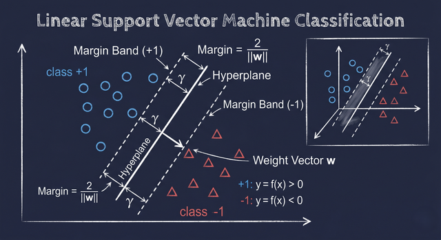
where: R = max ‖xᵢ‖ (max input norm)
γ = min yᵢ(w*ᵀxᵢ) / ‖w*‖ (functional margin) ✅ How to Use the Bound in Practice
subject to: yᵢ(wᵀxᵢ + b) ≥ 1 ∀i
Perceptron: finds any w: yᵢ(wᵀxᵢ + b) > 0 ∀i
Gen. bound ≈ O(√(VC·log(m)/m))
The Perceptron:
Mathematical Mastery
From First Principles
Every neural network — GPT, ResNet, BERT — is a stack of perceptrons wearing increasingly sophisticated clothes. If you can't derive the convergence proof, explain why XOR broke the field for a decade, and articulate the relationship between the Perceptron and SVMs, you don't yet have the mathematical foundations the rest of deep learning demands.
Read the Deep Dive ↓ Open the Math Lab 📐 w ← w + η(y − ŷ)x convergence ≤ (R/γ)² VC dim = d + 1 ŷ = sign(wᵀx + b) Table of Contents- Geometry of Hyperplanes & Decision Boundaries
- Perceptron Learning Algorithm (PLA)
- Novikoff's Convergence Theorem
- The XOR Problem & AI Winter
- Pocket Algorithm & Non-Separable Data
- Kernel Perceptrons
- Perceptron vs SVM: Margin Maximization
- VC Dimension & Statistical Theory
- From Perceptron to MLP: The Full Journey
01The Geometry of Hyperplanes and Decision Boundaries
Imagine you're a postal worker sorting mail in a giant warehouse. Your job: put blue envelopes on the left conveyor and red envelopes on the right. You draw a chalk line down the middle of the warehouse floor — everything blue lands left of the line, everything red lands right. Now scale that up: instead of a 2D floor, you have a 100-dimensional feature space, and instead of a chalk line, you have a hyperplane. That's what a perceptron does, geometrically.
A hyperplane in d-dimensional space is a (d-1)-dimensional subspace — a flat surface that divides the space into two half-spaces. In 2D, it's a line. In 3D, it's a plane. In 100D, it's a 99-dimensional surface. The perceptron's weight vector w is normal (perpendicular) to this hyperplane, and the bias b shifts it away from the origin. The decision function is simply: predict class +1 if wᵀx + b > 0, class -1 if wᵀx + b < 0.
Linear separability is the formal condition the perceptron requires: there must exist a hyperplane that perfectly separates the positive examples from the negative examples with some gap γ (called the margin). The margin γ is the minimum distance from any training point to the separating hyperplane. No margin, no convergence guarantee — as Novikoff's theorem will make precise. This geometric intuition is everything: all of Perceptron theory flows from asking "how does the algorithm find this hyperplane, and what happens if no such hyperplane exists?"
Decision function: ŷ = sign(wᵀx + b)Hyperplane: {x ∈ ℝᵈ : wᵀx + b = 0}
Margin γ: min_{i} y_i(wᵀx_i + b) / ‖w‖ 💡 Why the Bias Term Matters More Than You Think
Most introductions treat bias as an afterthought. In practice, it's critical — without a bias term, the hyperplane is forced to pass through the origin. This artificially constrains the solution space and will cause the algorithm to fail on problems that are separable by a hyperplane not passing through the origin. Always include bias. A common implementation trick: augment x with an extra dimension always set to 1, then absorb bias into the weight vector as the last component. This simplifies the math without losing generality.
02The Perceptron Learning Algorithm: Why the Update Rule Works
The Perceptron Learning Algorithm (PLA) is disarmingly simple and surprisingly deep. Initialize weights to zero (or random small values). For each training example, make a prediction. If the prediction is correct, do nothing. If it's wrong, update the weights using the rule: w ← w + η(y − ŷ)x. Repeat until all examples are correctly classified or a budget runs out.
Let's derive why this update makes geometric sense. When you misclassify a positive example (y = +1 but ŷ = -1), it means wᵀx < 0 — the weight vector is pointing away from x. The update adds ηx to w, rotating the weight vector toward x. When you misclassify a negative example (y = -1 but ŷ = +1), the update subtracts ηx from w, rotating the weight vector away from x. Each update makes a local correction that brings the current hyperplane closer to correctly classifying the misclassified point.
Here's the thing most tutorials miss about the learning rate η: unlike in gradient descent, it doesn't actually affect the convergence path of the basic Perceptron. Any positive η leads to the same sequence of weight vectors, just scaled differently. The reason: the sign activation function makes the convergence criterion purely directional — you care whether wᵀx is positive or negative, not its magnitude. η effectively just determines the step size of the rotation in weight space, but since only the direction of w matters (not its magnitude), η cancels out of the convergence analysis. You could set η = 1 for the basic PLA and lose nothing.
⚠️ Myth: The Perceptron Uses Gradient DescentThis is a widespread misconception. The perceptron's sign activation function has zero gradient almost everywhere and an undefined gradient at zero. You cannot apply gradient descent. The PLA is a direct rule derived from the geometry of the misclassification error, not from differentiating a loss function. It predates the backpropagation era and represents a different mathematical tradition — closer to online convex optimization than to the calculus-based learning that defines modern deep learning. This is exactly why moving to MLPs required replacing sign with smooth activation functions like sigmoid.
perceptron_pla.py — clean implementationimport numpy as np class Perceptron: def __init__(self, eta=1, max_iter=1000): self.eta = eta # learning rate (doesn't affect path) self.max_iter = max_iter def fit(self, X, y): # Augment X with bias column (all ones) n, d = X.shape Xb = np.column_stack([X, np.ones(n)]) self.w = np.zeros(d + 1) for t in range(self.max_iter): errors = 0 for xi, yi in zip(Xb, y): y_hat = np.sign(self.w @ xi) if y_hat != yi: # misclassification self.w += self.eta * yi * xi # w ← w + η(y−ŷ)x errors += 1 if errors == 0: break # converged! self.iterations_ = t + 1 return self def predict(self, X): Xb = np.column_stack([X, np.ones(len(X))]) return np.sign(Xb @ self.w)
03Novikoff's Convergence Theorem: The Proof That PLA Terminates
Novikoff's theorem is the mathematical backbone of the Perceptron. It proves that if your data is linearly separable, the PLA will always find a separating hyperplane — and gives you an explicit bound on how many updates it takes. The bound is (R/γ)², where R is the maximum norm of any input vector (how far points can be from the origin) and γ is the margin (minimum distance from any point to the optimal separating hyperplane, normalized by the weight norm).
The proof works by tracking two quantities simultaneously. First, it shows that the dot product of the current weight vector w(t) with the optimal weight vector w* grows at least linearly with the number of updates t: w(t)·w* ≥ γt. Second, it shows that the squared norm of w(t) grows at most linearly: ‖w(t)‖² ≤ R²t. Since the cosine of the angle between w(t) and w* must be ≤ 1, and this cosine is bounded by the ratio of the above quantities, you get t ≤ (R/γ)². Elegant and tight.
The practical implications are profound. First, the bound is independent of the number of training examples — it depends only on geometry (R and γ), not on dataset size. A linearly separable problem with 10 points and a small margin might take more iterations than a problem with 10 million points and a large margin. Second, the bound is tight — there exist datasets that require exactly (R/γ)² updates. Third, and most importantly: the theorem says nothing about non-separable data. If your data isn't linearly separable, the PLA will cycle forever, making the same sequence of updates repeatedly, never converging.
Novikoff's Bound: updates T ≤ (R/γ)²where: R = max ‖xᵢ‖ (max input norm)
γ = min yᵢ(w*ᵀxᵢ) / ‖w*‖ (functional margin) ✅ How to Use the Bound in Practice
Novikoff's bound tells you how to improve convergence speed: (1) normalize your inputs to reduce R — if all features have unit norm, R = 1, minimizing the numerator. (2) Ensure your problem has a large margin γ — the denominator. In practice, if PLA takes thousands of iterations on a supposedly separable dataset, check whether your data is actually linearly separable (no overlapping classes), and whether your features are on wildly different scales (inflating R). The bound guides both diagnosis and intervention.
04XOR and the First AI Winter: When One Line Isn't Enough
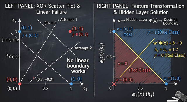
In 1969, Marvin Minsky and Seymour Papert published "Perceptrons" — a book that sent the AI field into what would become its first prolonged winter. Their central result: a single-layer perceptron cannot solve the XOR (exclusive-or) problem. XOR takes two binary inputs and returns 1 if exactly one input is 1, and 0 otherwise. Plot the four input-output pairs and you'll immediately see the problem: the two "1" outputs appear at (0,1) and (1,0), and the two "0" outputs at (0,0) and (1,1). No single straight line can separate these two classes.
The XOR problem represents a class of non-linearly separable problems — data configurations where no hyperplane can achieve zero training error. Minsky and Papert proved this for XOR and extended the critique to many other practically important functions, arguing (somewhat unfairly, in retrospect) that perceptrons were fundamentally limited. Their book was widely interpreted as proving that neural networks were a dead end, which contributed to a decade of dramatically reduced funding and research in the field.
The resolution — which would come 17 years later with the rediscovery of backpropagation — is to add layers. Two layers of perceptrons with nonlinear activations can solve XOR: the first layer creates new features that are linearly separable, and the second layer classifies in that new feature space. This is the core insight of multi-layer networks. XOR wasn't proof that neural networks were useless; it was proof that a single perceptron was insufficient and pointed directly toward the architecture that would eventually work.
🔴 The Minsky-Papert Critique Was OverextendedHere's the historical nuance that most ML courses gloss over: Minsky and Papert's mathematical results were correct. Their interpretation — that this killed the neural network approach — was not. The book analyzed single-layer perceptrons, not multi-layer ones. The mathematical machinery for training multi-layer networks (backpropagation) was known but not widely appreciated until Rumelhart, Hinton, and Williams published their famous 1986 paper. The AI Winter was partly a sociological phenomenon amplified by the rhetoric around a correct but narrowly-scoped mathematical result.
05The Pocket Algorithm: Handling the Real World's Messy Data
Real-world classification problems are almost never perfectly linearly separable. Label noise, measurement error, overlapping class distributions — in practice, you'll almost always have at least some misclassified points no matter where you put your hyperplane. The standard PLA response to this is to cycle endlessly without converging.
The Pocket Algorithm is the pragmatic fix. The name comes from the intuition: the algorithm runs the standard PLA but keeps its "best weights so far" in its pocket. After each update, it evaluates the current weight vector on the full training set. If the current weights correctly classify more examples than the pocket weights, it replaces the pocket. After a fixed number of iterations (your budget), it returns the pocket weights — the best it found, not necessarily the last. This guarantees that you get the best linearly-achievable solution even when the data isn't linearly separable.
The Pocket Algorithm is the foundation of an important principle in machine learning: tracking the best solution seen during optimization is almost always better than tracking the final solution. This idea resurfaces in modern deep learning as "best model checkpoint" — saving the model state at the lowest validation loss during training, not the model state at the end of training. Pocket → checkpointing: the same insight, 40 years apart.
💡 Pocket Algorithm = Prototype of Best-Model CheckpointingThe pocket algorithm's "save the best" heuristic predates early stopping and model checkpointing by decades. The reason it works: optimization algorithms are guaranteed to make progress toward the objective (fewer misclassifications) on the current step, but this doesn't mean the most recent weights are the best seen. Noisy updates, saddle points, and local minima can all cause temporary regression. Keeping a running best is essentially free (one extra copy of weights) and often dramatically improves final performance. This principle is now so fundamental to deep learning that it's built into every major training framework via model checkpoint callbacks.
06Kernel Perceptrons: Non-Linear Boundaries Without Explicit Features
The Kernel Perceptron extends the basic algorithm to learn non-linear decision boundaries — without explicitly computing coordinates in the high-dimensional feature space where the data would be linearly separable. This is the famous kernel trick, applied to the perceptron.
The key observation is the dual representation: the final weight vector w can always be written as a linear combination of the training examples that were misclassified: w = Σᵢ αᵢyᵢxᵢ, where αᵢ counts how many times example i was involved in an update. This means every prediction can be written as ŷ = sign(Σᵢ αᵢyᵢ xᵢᵀx) — entirely in terms of inner products between examples. Now replace the inner product xᵢᵀx with a kernel function K(xᵢ, x) = φ(xᵢ)ᵀφ(x), and you implicitly compute the inner product in the high-dimensional feature space φ(x) without ever computing φ(x) explicitly.
With the RBF (Gaussian) kernel K(xᵢ, x) = exp(-γ‖xᵢ - x‖²), the perceptron can learn decision boundaries of arbitrary complexity. The computational cost is O(n) per prediction (one kernel evaluation per training example), compared to O(d) for the standard perceptron. For very high-dimensional feature spaces (infinite-dimensional for the RBF kernel), this is dramatically more efficient. The kernel perceptron is theoretically satisfying and historically important — it prefigures the kernel SVM that would become dominant in the pre-deep-learning era.
🔬 The Dual Representation Is Not Just a TrickUnderstanding the dual form of the perceptron reveals something deep: the decision boundary is completely determined by a small subset of training examples — those that were ever misclassified during training. The rest of the training data is irrelevant to the final classifier. This is a precursor to the concept of "support vectors" in SVMs, where only the examples nearest the decision boundary determine the final model. The dual representation is fundamental, not a mathematical curiosity.
07Perceptron vs SVM: Why Margin Maximization Changes Everything
The Perceptron and the Support Vector Machine (SVM) both find linear separating hyperplanes for linearly separable data. But the Perceptron finds any separating hyperplane — wherever it happens to converge to — while the SVM finds the optimal one: the maximum margin hyperplane.
The functional margin of a hyperplane is min_i y_i(wᵀxᵢ + b) — how confidently the current weights classify the closest point. The geometric margin normalizes this by ‖w‖ to get a distance in input space. The SVM solves the optimization problem of maximizing this geometric margin subject to the constraint that all points are correctly classified. The solution is unique (the optimization problem is convex) and corresponds to the hyperplane equidistant from the nearest positive and negative examples — the "support vectors."
Why does margin matter? The VC theory tells us that for a fixed hypothesis class, the maximum margin classifier has the best generalization bounds — the smallest expected difference between training error and test error. A Perceptron that barely separates the training data (small margin) is likely to fail on test points near the boundary. An SVM that maximizes the margin is maximally confident in its decision boundary and has better theoretical guarantees on unseen data. This is the fundamental reason SVMs dominated classification before deep learning: they found the most defensible linear classifier, not just any linear classifier.
SVM objective: maximize γ = 1/‖w‖subject to: yᵢ(wᵀxᵢ + b) ≥ 1 ∀i
Perceptron: finds any w: yᵢ(wᵀxᵢ + b) > 0 ∀i
08VC Dimension and Statistical Learning Theory
The Vapnik-Chervonenkis (VC) dimension is the fundamental measure of a hypothesis class's complexity — how many different binary labelings of a dataset the class can implement. For the Perceptron in d-dimensional space, the VC dimension is exactly d + 1. This means a d-dimensional perceptron can shatter (correctly classify in all 2^(d+1) possible ways) any set of d+1 points in general position, but cannot shatter any set of d+2 points.
The VC dimension directly bounds generalization via the fundamental theorem of statistical learning: with probability at least 1-δ over a training set of size m, the true error of any perceptron trained to zero training error is bounded by train_error + O(√((d·log(m/d) + log(1/δ)) / m)). This tells you: more dimensions → higher capacity → need more data to generalize. A perceptron in 1000-dimensional space needs roughly 1000 times as many training examples as a perceptron in 1-dimensional space to achieve the same generalization guarantee, holding everything else equal.
The bias-variance perspective: the Perceptron is a high-bias, low-variance model. "High bias" means it makes strong assumptions about the data (linear separability), causing systematic underfitting when that assumption is wrong. "Low variance" means its predictions are stable across different training sets because it has few degrees of freedom (d+1 parameters). This makes it reliable and robust to overfitting but fundamentally limited in representational power. Understanding this tradeoff is the first step to understanding why deep networks — with their enormous VC dimensions — require massive datasets and careful regularization.
09From Perceptron to MLP: The Three Changes That Unlocked Deep Learning
The Multi-Layer Perceptron (MLP) is the direct architectural descendant of the single-layer perceptron. Three changes transform one into the other — and each change is driven by a specific mathematical necessity.
Change 1: Multiple layers. Stack perceptrons: the output of one layer feeds as input to the next. This gives the network the ability to learn hierarchical representations — the first layer learns low-level features, subsequent layers combine them into higher-level abstractions. The mathematical result: MLPs are universal function approximators for any continuous function on a compact domain (universal approximation theorem), whereas single-layer perceptrons can only learn linear functions.
Change 2: Differentiable activations. Replace sign(x) with sigmoid, tanh, or ReLU. Sign's zero gradient makes backpropagation impossible — you can't propagate error signals backward through a function with no derivative. Sigmoid and tanh are smooth and differentiable everywhere. ReLU (max(0,x)) has zero gradient for negative inputs but is differentiable for positive inputs, which is sufficient for practical training. This single change enables gradient-based optimization of the entire multi-layer network.
Change 3: Backpropagation. Efficiently compute gradients of the loss function with respect to every weight in the network using the chain rule. Without backpropagation, training a 10-layer network would require computing gradients for each weight individually — computationally infeasible. With it, you do one forward pass and one backward pass, and all gradients are available simultaneously. Backpropagation is the algorithm; gradient descent is the optimization method; differentiable activations are the prerequisite. All three together, standing on the Perceptron's shoulders.
✅ The Perceptron's Legacy in Modern NetworksThe Transformer architecture that powers GPT, BERT, and Claude is fundamentally a stack of linear transformations (perceptrons) with nonlinear activations (ReLU/GELU) and an attention mechanism. The "feed-forward" sublayer in every Transformer block is literally a two-layer MLP applied independently to each position. Every time you use a language model, you're using a massively scaled version of the mathematics Frank Rosenblatt first described in 1958. The perceptron didn't fail — it became the atom from which all modern neural architectures are built.
synthesisHow It All Connects: The Perceptron's Full Arc
The Perceptron's story is one of the most instructive in all of machine learning. It starts with a geometric intuition (separating hyperplane), gains mathematical rigor through the PLA and Novikoff's theorem, hits a fundamental limitation (XOR), spawns pragmatic solutions (Pocket Algorithm, Kernel Trick), informs better algorithms (SVM via margin maximization), grounds theoretical understanding (VC dimension, bias-variance), and ultimately seeds the architecture that would transform the world (MLP → deep networks). Each concept is a building block; together they constitute the mathematical foundation of neural computation.
The lesson isn't just historical. When you understand why the sign activation can't be used in a multi-layer network, you understand why we use ReLU. When you understand VC dimension, you understand why larger models need more data. When you understand margin maximization, you understand why data augmentation and regularization help. The Perceptron is not a quaint historical artifact — it's a lens for understanding every modern ML system.
getting startedMastery Roadmap: From PLA to MLP in Python
perceptron_mastery_path.py# Step 1: Implement PLA from scratch (understand the update rule)
# Step 2: Test on linearly separable data, verify Novikoff bound
# Step 3: Test on XOR — watch it fail to converge
# Step 4: Implement Pocket Algorithm for noisy data
# Step 5: Implement Kernel Perceptron with RBF kernel
# Step 6: Compare to sklearn SVM — visualize margin difference
from sklearn.datasets import make_blobs, make_circles
from sklearn.svm import SVC
import numpy as np
# Generate linearly separable data
X, y = make_blobs(n_samples=100, centers=2, cluster_std=0.5, random_state=42)
y = 2 * y - 1 # map {0,1} → {-1,+1}
# Estimate margin and verify Novikoff bound
svm = SVC(kernel='linear', C=1e6).fit(X, y)
w_star = svm.coef_[0]
gamma = 1 / np.linalg.norm(w_star) # geometric margin
R = np.max(np.linalg.norm(X, axis=1)) # max input norm
novikoff_bound = (R / gamma) ** 2
print(ff"Novikoff bound: {novikoff_bound:.0f} updates")
# Train our Perceptron and compare
pla = Perceptron().fit(X, y)
print(ff"PLA actual updates: {pla.iterations_}")
# Should be ≤ novikoff_bound ✓
# Now test XOR — should loop indefinitely (cap at max_iter)
X_xor = np.array([[0,0],[0,1],[1,0],[1,1]])
y_xor = np.array([-1, 1, 1, -1])
pla_xor = Perceptron(max_iter=100).fit(X_xor, y_xor)
preds = pla_xor.predict(X_xor)
print(ff"XOR accuracy: {(preds==y_xor).mean():.0%}") # <100%
FAQFrequently Asked Questions
Does the Perceptron use gradient descent? + No. This is one of the most common misconceptions in ML education. The sign activation function used in the standard Perceptron has zero gradient almost everywhere and an undefined gradient at exactly zero. Gradient descent requires a differentiable loss function — the Perceptron update rule cannot be derived this way. The PLA update is derived geometrically: when a misclassification occurs, the weight vector is updated to move the decision boundary toward correctly classifying the misclassified point. This makes the Perceptron more closely related to online convex optimization and coordinate descent than to gradient descent. The switch to gradient-based learning is what motivated replacing the sign function with differentiable activations (sigmoid, tanh, ReLU) in Multi-Layer Perceptrons. What does Novikoff's theorem actually guarantee? + Novikoff's theorem guarantees that if a dataset is linearly separable with functional margin γ and all input vectors have norm at most R, the Perceptron Learning Algorithm will converge in at most (R/γ)² weight updates, regardless of the order in which training examples are presented (in the most general version). This is a worst-case bound, not an average-case guarantee. It's independent of the number of training examples — only the geometric properties of the data matter. Crucially, the theorem says nothing about non-separable data: if the data isn't linearly separable, the algorithm will cycle indefinitely without converging. Why can't a single Perceptron solve XOR? + The XOR function produces class 1 for inputs (0,1) and (1,0), and class 0 for (0,0) and (1,1). If you plot these four points in 2D, the two class-1 points and two class-0 points appear in alternating corners of a square. There is no straight line that can separate these two classes — the data is not linearly separable. Since a single Perceptron can only implement a linear decision boundary (a hyperplane in feature space), it cannot represent the XOR function for any setting of its weights. This requires at least two layers: a hidden layer that transforms the feature space, and an output layer that classifies in the transformed space. What is the VC dimension of a Perceptron? + The VC dimension of a Perceptron (with bias) in d-dimensional input space is exactly d+1. This means a d-dimensional Perceptron can shatter (correctly classify in all 2^(d+1) possible ways) any set of d+1 points in general position, but cannot shatter any set of d+2 points. The VC dimension tells you the complexity of the hypothesis class and bounds the generalization error: a larger VC dimension means higher capacity (can represent more functions), which means you need more training data to reliably generalize. This is why high-dimensional Perceptrons require more data than low-dimensional ones, all else equal. What is the difference between a Perceptron and an SVM? + Both are linear classifiers that find a hyperplane separating two classes. The key difference is which hyperplane they find. The Perceptron finds any hyperplane that correctly separates the classes — whatever it converges to, which depends on the initial weights and the order of training examples. The SVM finds the unique optimal hyperplane: the maximum margin hyperplane, equidistant from the nearest positive and negative examples (the support vectors). The SVM's solution is deterministic, order-independent, and has the best theoretical generalization guarantees of any linear classifier. The Perceptron is computationally simpler but produces inferior generalization bounds and non-unique solutions. How does the learning rate affect Perceptron convergence? + Counterintuitively, for the standard binary Perceptron on linearly separable data, the learning rate η does not affect the convergence path — only the scale of the weight vector. This is because the sign activation function makes the prediction depend only on the sign of wᵀx, not its magnitude. Scaling w by any positive constant doesn't change any prediction. Therefore, multiplying all weight updates by η is equivalent to rescaling the entire weight vector by η — which doesn't change which examples are misclassified or the order in which updates occur. The number of updates before convergence is independent of η. This changes for gradient-based learners (like MLPs) where η dramatically affects convergence speed and stability. What is the Pocket Algorithm and when should I use it? + The Pocket Algorithm is a modification of the PLA for non-linearly separable data. It runs the standard PLA update rule but keeps track of the best weight vector seen so far (the one with the lowest training error). After a fixed budget of iterations, it returns the "pocket weights" rather than the current weights. Use the Pocket Algorithm when: your data has label noise (some examples are incorrectly labeled), your data has overlapping class distributions (classes aren't perfectly separable), or you want a linear classifier as a fast baseline when you can't be sure of separability. It's particularly useful as a component of boosting algorithms and for problems where a linear classifier is sufficient but perfection is impossible. How does the Kernel Perceptron work without explicit feature computation? + The Kernel Perceptron exploits the dual representation of the Perceptron: the final weight vector can always be written as w = Σᵢ αᵢyᵢxᵢ — a linear combination of the training examples. Predictions become ŷ = sign(Σᵢ αᵢyᵢ xᵢᵀx) — entirely in terms of inner products between examples. The kernel trick replaces xᵢᵀx with a kernel function K(xᵢ, x) = φ(xᵢ)ᵀφ(x), implicitly computing inner products in a high-dimensional feature space without ever computing φ(x) explicitly. The RBF kernel K(xᵢ, x) = exp(-γ‖xᵢ-x‖²) corresponds to an infinite-dimensional feature space, enabling the Kernel Perceptron to learn arbitrarily complex decision boundaries while retaining the simple PLA update rule.📐 Perceptron Math Lab
Four interactive experiments: run the PLA, verify Novikoff's bound, test XOR, and explore VC dimension.
Click to add points (left click = class +1, right click = class -1) · Watch PLA find the boundary
PLA SimulatorClick to add data points. Left click = blue (+1), right click = red (−1). Then run the Perceptron Learning Algorithm to watch it find the decision boundary.
Learning rate η 1.0 0 Iterations 0 Current errors — Weight vector Idle StatusNote: Try different η values — notice they all converge to the same boundary, confirming Novikoff's theorem that η doesn't affect the convergence path.
Actual PLA updates vs Novikoff bound (R/γ)² across margin sizes
Novikoff Bound Explorer Margin size γ 0.30 Max norm R 2.0 Dataset size n 50 — (R/γ)² bound — Actual updates — Actual / Bound — Theorem holds?As γ decreases (smaller margin), the bound (R/γ)² increases quadratically. Notice that actual updates are always ≤ the bound — confirming Novikoff's theorem.
XOR data — blue = class +1, red = class −1 · Watch PLA fail to converge
XOR Non-Separability Demo Problem Type Cycle Detection 0 Iterations 100% Best error — Separable? Idle PLA statusShattering demonstration: all 2ⁿ labelings for n points · VC dim = d+1 for Perceptron
VC Dimension Explorer Dimensions d 2 Training examples m 100 d+1 VC Dimension — Max labelings — Gen. error bound — Data for 5% bound VC dim = d+1 = 3Gen. bound ≈ O(√(VC·log(m)/m))
Keep reading
Related articles
 AI
AIEnterprise RAG: How to Build Accurate, Private AI Systems | Zetsapp
Teams frequently ask "should we fine-tune or use RAG?" as if it's binary. In production, the strongest systems use both: RAG for dynamic factual grounding, and light fine-tuning (or just careful prompting) for output style, tone, and domain-specific reasoning patterns. Don't fine-tune to teach the model facts — that's what retrieval is for.
 AI
AIAI Agents for Business: Use Cases, Implementation Guide & ROI in 2026 | Zetsapp
The most common mistake in discovery calls is a stakeholder describing a chatbot project using agent language ("it should be smart and handle anything"). Before scoping anything, get explicit about which systems the agent needs write access to. If the answer is "none, it just answers questions," you likely need a well-grounded RAG chatbot, not an agent — simpler, cheaper, faster.
 AI
AIThe Shift to Cloud 3.0: Architecting Low-Latency Apps With Distilled On-Device AI | Zetsapp
The Shift to Cloud 3.0: Architecting Low-Latency Apps With On-Device AI :root { --sp: 0.28s; } [data-theme="dark"]…