The Attention Mechanism: Heart of Every Transformer

The Attention Mechanism — Deep Dive · 4,200 words · 4 interactive labs · April 2026

The Attention Mechanism:
Heart of Every Transformer

Queries. Keys. Values. Masking. Multi-head attention. The mechanism that made the 2017 paper "Attention Is All You Need" one of the most cited in all of AI — explained from first principles, with interactive labs you can manipulate right now.

Read the Deep Dive ↓ Open the Lab ⚗️ Table of Contents

1. Why Attention Exists
2. Queries & Keys: Asking and Answering
3. The Attention Pattern & Softmax
4. Masking: The Training Trick
5. Values: Actually Updating Embeddings
6. Multi-Head Attention
7. Parameter Count: Where 58B Go
8. Getting Started: Code It Yourself

01Why Attention Exists: The Word "Mole" Changes Everything

Here's a question that should feel obvious but actually isn't: when you read the sentence "take a biopsy of the mole," how do you know which kind of mole that is? Not the animal, not the chemistry unit — the skin lesion. You know because of context. The word "biopsy" earlier in the sentence made it immediately clear. Your brain didn't process each word in isolation; it wove everything together into a coherent meaning.

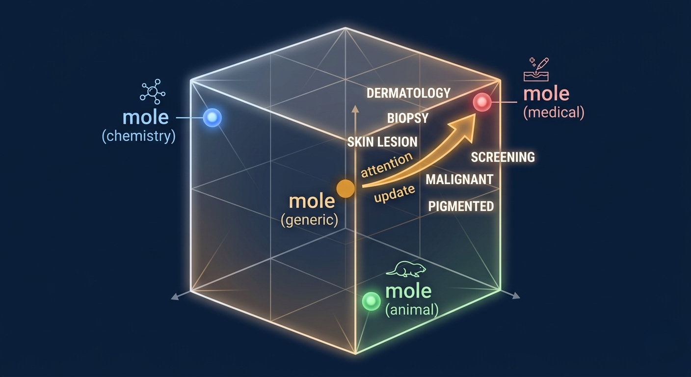
This is exactly the problem that the attention mechanism was invented to solve. After the first step of a transformer — tokenization and initial embedding — every token gets a vector, but that vector encodes only the bare meaning of the word itself, with no context whatsoever. The embedding for "mole" is identical whether you're talking about chemistry, animals, or dermatology. The attention block is the mechanism that fixes this: it lets embeddings update themselves based on what surrounds them.

Picture this more concretely. In high-dimensional embedding space, there might be three distinct "directions" corresponding to the three meanings of mole — a chemistry direction, an animal direction, a medical direction. The initial embedding lands somewhere generic. The attention block's job is to compute exactly what should be added to that generic vector to shift it toward the correct specific direction, based on the surrounding context. That addition is the output of attention. Everything else — queries, keys, values, masking, multiple heads — is the machinery that computes it.

💡 The Key Intuition: Attention is Contextual Embedding Updating

Attention doesn't create new information from thin air. It routes existing information from one position in the sequence to another. Think of each token as a node in a graph, with attention weights determining how much each node "receives" from every other node. High attention weight = strong connection = more information transfer. The output of attention is just the original embeddings plus a context-informed correction.

---

02Queries & Keys: The Question-Answer System Inside Every Head

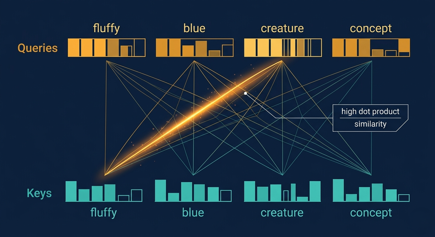
The mechanism that determines which tokens should influence which other tokens is the query-key system, and it's one of the most elegant ideas in modern deep learning. Every token in the sequence generates two vectors simultaneously: a query and a key. The query says "I'm looking for something like this." The key says "I can offer something like this." Compatibility is measured by how well they match.

Concretely: take the example "a fluffy blue creature roamed the verdant forest." If an attention head is trying to help adjectives update their corresponding nouns, then the noun "creature" would produce a query vector that encodes something like "I'm a noun, looking for preceding adjectives." The words "fluffy" and "blue" would produce key vectors that encode "I'm an adjective, in a position before nouns." How well these match — how much the query and key align — determines the attention weight. The alignment is measured with a dot product: when two vectors point in similar directions in the query-key space, their dot product is large and positive, meaning strong attention.

Here's the thing most tutorials miss: the query and key matrices map embeddings into a much smaller space — 128 dimensions in GPT-3, down from 12,288. This isn't just an efficiency trick. It's a compression that forces the model to distill each token's embedding into the single most relevant aspect for this particular attention head — "am I a noun looking for adjectives?" vs. "am I an adjective that a noun should attend to?" The full embedding is too rich; the query-key compression focuses it.

🔥 Common Mistake: Thinking Q/K Must Be Interpretable

In practice, the query and key matrices don't learn to encode things as clean as "noun looking for adjective." They learn whatever compression of the embeddings best reduces training loss — which is often far messier and harder to interpret. The adjective-noun example is a useful teaching analogy, not a description of what actually happens. When researchers probe real attention heads, they often find behaviors like "previous-word attention," "first-token attention," or "copy behavior" — not clean grammatical roles.

query_key.py

import torch
import torch.nn as nn
import math

class AttentionHead(nn.Module):
 def __init__(self, d_model=12288, d_head=128):
 super().__init__()
 # Query and Key matrices: d_model → d_head
 self.W_Q = nn.Linear(d_model, d_head, bias=False)
 self.W_K = nn.Linear(d_model, d_head, bias=False)

 def attention_scores(self, embeddings):
 # embeddings: (seq_len, d_model)
 Q = self.W_Q(embeddings) # (seq_len, d_head) — queries
 K = self.W_K(embeddings) # (seq_len, d_head) — keys

 # Dot product of all Q-K pairs: (seq_len, seq_len)
 # Scale by sqrt(d_head) for numerical stability
 scores = Q @ K.transpose(-2, -1) / math.sqrt(self.d_head)

 # scores[i][j] = how much token i attends to token j
 return scores # raw logits, before softmax

---

03The Attention Pattern: A Grid of Relevance

Once you have query and key vectors for every token in the sequence, you compute the dot product between every possible query-key pair. For a sequence of N tokens, this produces an N×N grid of raw scores — one score for each pair of positions. The score at row i, column j says "how relevant is token j to token i?" Large positive score: j strongly influences i. Small or negative score: j is irrelevant to i. These raw scores can be any real number, which is why the next step is necessary.

Apply softmax column-by-column. Each column now sums to 1.0 and all values are between 0 and 1 — it's now interpretable as a probability distribution: "given token i, what fraction of its update should come from each other token?" This normalized N×N grid is what's called the attention pattern. It's the fingerprint of what an attention head has decided to focus on, and it's where a lot of interpretability research happens — visualizing attention patterns can reveal fascinating (and sometimes confusing) structures in what the model has learned.

A small but important detail from the original paper: before softmax, you divide all dot product scores by √d_head (the square root of the query-key dimension). This prevents the dot products from growing so large that the softmax output becomes almost binary — all weight on one token, none on others — which would make the gradients vanish during training. It's one of those numerical stability tricks that looks arbitrary in the formula but is crucial in practice.

🔮 Myth: High Attention = High Importance

Visualizing attention patterns is tempting as a model interpretation tool — but high attention weight doesn't cleanly correspond to semantic importance. Research by Jain & Wallace (2019) found that attention weights are not reliable explanations of predictions. A token can receive high attention for purely mechanical reasons (like being the first token, which GPT models often attend to heavily by default). True interpretability requires probing beyond attention weights.

attention_pattern.py

import torch
import torch.nn.functional as F
import math

def attention_pattern(Q, K, mask=None):
 """
 Q: (seq, d_head)
 K: (seq, d_head)
 Returns: attention weights (seq, seq) — each column sums to 1
 """
 d_head = Q.shape[-1]
 # Raw dot product scores: (seq, seq)
 scores = Q @ K.T / math.sqrt(d_head)

 # Apply causal mask if provided
 if mask is not None:
 scores = scores.masked_fill(mask == 0, -float('inf'))

 # Softmax along dimension 1 (over key positions)
 weights = F.softmax(scores, dim=1)
 return weights # N×N grid of attention weights

# Example: 5 tokens, d_head=4
Q = torch.randn(5, 4)
K = torch.randn(5, 4)
w = attention_pattern(Q, K)
print("Each column sums to 1:", w.sum(dim=1)) # → [1., 1., 1., 1., 1.]

---

04Masking: Why Tokens Can't Look Into the Future

Here's a training efficiency insight that changes the entire structure of how transformers work. When you train on a sequence of N tokens, you could treat it as N separate training examples — predict token 2 from token 1, predict token 3 from tokens 1-2, etc. That would be inefficient. Instead, transformers make all N predictions simultaneously in a single forward pass: position 1 predicts what comes at position 2, position 2 predicts position 3, and so on, all at once. This gives you N training signals from one forward pass.

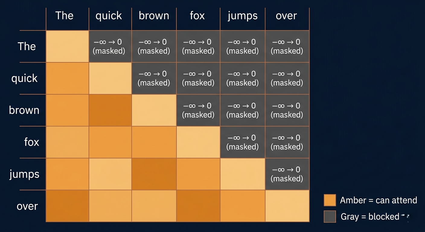
The problem: if position 5 can attend to position 8 during training, it "sees the answer" for predicting what comes after position 5. That's cheating — and it would make the model useless at inference time, when future tokens literally don't exist yet. The solution is masking: before applying softmax to the attention pattern, set all "future-looking" entries to negative infinity. After softmax, these become exactly zero. Each position can only attend to itself and positions before it.

The clever detail: setting to -∞ rather than 0 before softmax ensures the remaining weights still normalize correctly. If you just zeroed out the future entries after softmax, the remaining weights wouldn't sum to 1 anymore. Setting to -∞ first, then applying softmax, produces exactly the right behavior: future positions are impossible to attend to, and the weights over available positions still form a valid probability distribution.

✅ Masking at Inference vs Training

The mask is applied during both training and inference in GPT-style models. At inference (chatting), you're always predicting the next token from what you have, so the mask is already naturally satisfied — you never have future tokens. But the implementation applies masking uniformly regardless, which means the code path is the same in both modes. This simplifies the codebase: no special-casing for "am I training or inferring?" The mask is always there.

causal_mask.py

import torch

def causal_mask(seq_len):
 """
 Creates a lower-triangular mask.
 True = can attend, False = blocked (set to -inf before softmax)
 """
 # Lower triangular matrix of 1s
 mask = torch.tril(torch.ones(seq_len, seq_len))
 return mask.bool()

mask = causal_mask(5)
print(mask.int())
# tensor([[1, 0, 0, 0, 0], ← token 0: only attends to itself
# [1, 1, 0, 0, 0], ← token 1: attends to 0,1
# [1, 1, 1, 0, 0], ← token 2: attends to 0,1,2
# [1, 1, 1, 1, 0],
# [1, 1, 1, 1, 1]]) ← token 4: attends to all

# Apply to scores: blocked positions become -inf
scores_masked = scores.masked_fill(~mask, float('-inf'))
weights = torch.softmax(scores_masked, dim=-1)
# Future positions: 0.0000 — can't attend to future

---

05Values: Actually Moving Information Between Embeddings

The attention pattern tells you which tokens should influence which others, and by how much. But it doesn't tell you what to transfer. That's the job of the value map. Once you know that "creature" should strongly attend to "fluffy" and "blue," you still need to know: what exactly should be extracted from "fluffy's" embedding and added to "creature's" embedding? That's the value vector — a specific addition to the target embedding, computed from the source token.

The value map is implemented as a matrix (or more precisely, a factored pair of matrices) that you multiply by the source embedding. For "fluffy," the value vector is something like "this is what to add to nouns — a direction in embedding space that encodes fluffiness." For "blue," it's a direction encoding color. These value vectors live in the full 12,288-dimensional embedding space, not the compressed 128-dimensional query-key space. The update to "creature" is then a weighted sum: large weight × fluffy's value vector + large weight × blue's value vector + small weights × everyone else's value vectors. Add this sum to the original "creature" embedding and you get a more contextually enriched vector.

The factored value matrix deserves attention. In practice, the value map is split into a "value down" matrix (embedding → 128-dim) and an "output" matrix (128-dim → embedding), keeping it the same parameter count as the query and key matrices. The combined effect is a low-rank linear transformation — it can't represent arbitrary transformations of the full embedding space, but the constraint is a feature: it regularizes what information can be transferred, preventing the model from doing arbitrary computation in a single head. Each head specializes.

💡 The Value Map's Real Intuition

Ask yourself: if word X is attending to word Y, what should X "receive" from Y? The value map answers this. For our adjective-noun example, "fluffy's" value map output for "creature" might be a vector that adds fluffiness-related directions. But the value map is learned — it finds whatever additive correction best helps predict the next token. In practice, value maps sometimes encode things like "copy this token's identity" or "negate this embedding direction" — again, far messier than clean grammatical abstractions.

values_update.py

import torch
import torch.nn as nn

class SingleAttentionHead(nn.Module):
 def __init__(self, d_model=768, d_head=64):
 super().__init__()
 self.d_head = d_head
 self.W_Q = nn.Linear(d_model, d_head, bias=False)
 self.W_K = nn.Linear(d_model, d_head, bias=False)
 # Value: factored as V_down (d_model→d_head) and V_up (d_head→d_model)
 self.W_V_down = nn.Linear(d_model, d_head, bias=False)
 self.W_V_up = nn.Linear(d_head, d_model, bias=False)

 def forward(self, x, mask=None):
 # x: (seq, d_model)
 Q, K = self.W_Q(x), self.W_K(x)
 # Attention weights: (seq, seq)
 scores = (Q @ K.T) / (self.d_head ** 0.5)
 if mask is not None:
 scores = scores.masked_fill(~mask, -1e9)
 attn = scores.softmax(dim=-1) # (seq, seq)

 # Value vectors (compressed): (seq, d_head)
 V_down = self.W_V_down(x)
 # Weighted sum: for each position, mix value vectors by attention weight
 mixed = attn @ V_down # (seq, d_head)
 # Project back to full embedding space
 delta_e = self.W_V_up(mixed) # (seq, d_model)
 return x + delta_e # residual connection

---

06Multi-Head Attention: 96 Conversations Happening Simultaneously

A single attention head can capture one type of contextual relationship — maybe adjectives updating nouns. But language is far richer than that. "Harry" should attend to "Potter" to resolve identity, to "wizard" to infer the universe, to "killed" to understand narrative context, and to "the Chosen One" to understand mythological framing — all simultaneously, all different types of relationships, all relevant to correctly predicting the next token. This is why transformers use multi-head attention: many attention heads running in parallel, each with its own Q, K, and V matrices, each potentially learning a different kind of contextual relationship.

GPT-3 uses 96 attention heads per layer. Each head computes its own attention pattern and produces its own set of proposed changes to every embedding in the sequence. These 96 proposals are then summed together at each position, and added to the original embedding. The result: a single embedding position has simultaneously incorporated 96 different types of contextual information — whatever the 96 heads learned to specialize in during training. Crucially, each head operates on the same input embeddings but with completely independent parameters, so they can diverge into truly different specializations.

The counterintuitive result: even though attention "gets all the attention" as the iconic mechanism, it accounts for only about a third of GPT-3's 175 billion parameters. 96 heads × 96 layers × ~6.3 million parameters per head ≈ 58 billion parameters. The other ~117 billion live in the MLP blocks sitting between attention layers — the blocks that are often described as the "memory" of the model, storing factual associations. Attention routes information; MLPs store and transform it.

🔥 The O(n²) Scaling Problem

The attention pattern is N×N where N is the sequence length. Computing 96 of these per layer, across 96 layers, means the computation scales as O(n²) with sequence length. Double the context: 4× the attention compute. This is why extending context windows is hard — going from 2K to 128K tokens is not 64× more expensive, it's 4,096× more expensive in the attention layers alone. Flash Attention, sparse attention, and linear attention mechanisms are all attempts to tame this quadratic scaling. Understanding the N×N nature of the attention pattern makes these challenges immediately clear.

multi_head_attention.py

import torch
import torch.nn as nn

class MultiHeadAttention(nn.Module):
 def __init__(self, d_model=768, n_heads=12):
 super().__init__()
 self.n_heads = n_heads
 self.d_head = d_model // n_heads # 64 per head for GPT-2

 # All Q,K,V projections in one matrix each for efficiency
 self.W_Q = nn.Linear(d_model, d_model, bias=False)
 self.W_K = nn.Linear(d_model, d_model, bias=False)
 self.W_V = nn.Linear(d_model, d_model, bias=False)
 self.W_O = nn.Linear(d_model, d_model, bias=False) # output/value-up

 def forward(self, x, mask=None):
 B, T, C = x.shape # batch, seq_len, d_model
 H, D = self.n_heads, self.d_head

 # Project and split into heads: (B, T, H, D) → (B, H, T, D)
 Q = self.W_Q(x).view(B,T,H,D).transpose(1,2)
 K = self.W_K(x).view(B,T,H,D).transpose(1,2)
 V = self.W_V(x).view(B,T,H,D).transpose(1,2)

 # All heads in parallel: (B, H, T, T)
 scores = (Q @ K.transpose(-2,-1)) / (D**0.5)
 if mask is not None:
 scores = scores.masked_fill(~mask, -1e9)
 attn = scores.softmax(dim=-1) # (B,H,T,T)
 out = (attn @ V).transpose(1,2).reshape(B,T,C) # (B,T,C)
 return x + self.W_O(out) # residual

---

07Parameter Count: Where Those 58 Billion Attention Parameters Come From

Let's run the GPT-3 numbers. Each attention head has four matrices: W_Q (12,288 × 128), W_K (12,288 × 128), W_V_down (12,288 × 128), and contributes to W_O. Each of these four has 12,288 × 128 = 1,572,864 parameters. Four matrices = ~6.3 million parameters per head. GPT-3 uses 96 heads per layer and 96 layers. So the attention parameter total: 6.3M × 96 × 96 ≈ 58 billion.

What about the other 117 billion parameters? They live in the MLP blocks — the feed-forward layers sitting between each attention layer. Each MLP has two weight matrices expanding from d_model to 4×d_model and back. For GPT-3: 12,288 × 49,152 × 2 ≈ 1.2 billion parameters per MLP block, times 96 layers ≈ 115 billion. This is the majority of the model, and it's the part that's hardest to interpret — these are the blocks that seem to store world knowledge as distributed associations, not the attention blocks that route information around.

The practical takeaway: when people talk about "attention is all you need," they're referring to the mechanism's importance, not its parameter share. In terms of raw computation, the MLP blocks dominate. The attention mechanism is lightweight but critical — it's the routing system, not the storage. Remove attention and the model loses the ability to incorporate context. Remove MLPs and the model loses the ability to store complex knowledge. Both are essential, in different ways.

💡 Why GPT-3 Is Being Used As Reference Here

GPT-3's architecture was publicly disclosed in the original paper. Modern frontier models (GPT-4, Claude 3 Opus, Gemini Ultra) keep their architectural details secret. GPT-3 has a "charming authenticity" as the first model to genuinely capture mainstream attention, and every architectural insight from its documented numbers transfers directly to understanding its successors — the design philosophy is the same, just scaled differently.

---

08Getting Started: Run a Full Attention Layer in 50 Lines

The best way to cement your understanding of attention is to run it on real text and inspect the outputs. Here's a self-contained example using nanoGPT's attention implementation — everything from tokenization to attention pattern visualization.

attention_inspect.py

import torch
import matplotlib.pyplot as plt
import numpy as np

# Load a real GPT-2 model (smallest: 117M params)
from transformers import GPT2Model, GPT2Tokenizer

model = GPT2Model.from_pretrained('gpt2', output_attentions=True)
tokenizer = GPT2Tokenizer.from_pretrained('gpt2')
model.eval()

text = "The fluffy blue creature roamed the verdant forest"
inputs = tokenizer(text, return_tensors='pt')
tokens = tokenizer.convert_ids_to_tokens(inputs['input_ids'][0])

with torch.no_grad():
 outputs = model(**inputs)

# Extract attention patterns from layer 0, head 0
layer, head = 0, 4
attn_pattern = outputs.attentions[layer][0, head].numpy()

# Visualize the N×N attention grid
plt.figure(figsize=(8,6))
plt.imshow(attn_pattern, cmap='YlOrBr')
plt.colorbar(label='Attention weight')
plt.xticks(range(len(tokens)), tokens, rotation=45)
plt.yticks(range(len(tokens)), tokens)
plt.title(f'GPT-2 Attention Pattern — Layer {layer}, Head {head}')
plt.tight_layout()
plt.show()

synthesisHow It All Connects

The full attention mechanism in one breath: embed tokens into high-dimensional vectors → for each head, compute query vectors (what I'm looking for) and key vectors (what I can offer) → dot product every Q-K pair to get raw relevance scores → divide by √d_head for stability → apply causal mask (set future to −∞) → softmax to get normalized attention weights → compute value vectors from source embeddings → take weighted sums using attention weights → add back to original embeddings (residual connection). Run 96 of these in parallel, sum their outputs, and you have multi-head attention.

Repeat this across 96 layers, alternating with MLP blocks, and you have GPT-3. The deep stacking is what allows increasingly abstract representations to form: early layers might update simple grammatical relationships, later layers incorporate high-level semantic context — tone, genre, factual associations. The "murderer" in a mystery novel context lands in the final layer only because 96 attention layers worked together to pull relevant context from hundreds of pages earlier.

---

FAQFrequently Asked Questions

What's the difference between self-attention and cross-attention? + In self-attention, queries, keys, and values all come from the same sequence — tokens attending to tokens within the same passage. In cross-attention, queries come from one sequence (e.g., the target language being generated) while keys and values come from a different sequence (e.g., the source language input). Cross-attention is how original encoder-decoder transformers (for translation) worked. GPT-style models use only self-attention. Models like DALL-E that combine text and image use cross-attention between modalities. Why divide by √d_head in the attention score formula? + When d_head is large (say 128), the dot products between random vectors tend to have magnitude proportional to √d_head. Without scaling, these large values push the softmax into near-saturation — one value dominates and the rest get probability ≈ 0. This makes gradients vanish and training unstable. Dividing by √d_head keeps the dot products at unit scale on average, resulting in a softmax distribution that isn't degenerate. It's a single line of code with disproportionate impact on training stability. What do different attention heads actually learn to attend to? + Research by Elhage et al. at Anthropic and Olah et al. at OpenAI has found specific patterns in real models. Common behaviors include: "induction heads" (attend to the token that follows a previous occurrence of the current token — useful for copying patterns), "previous token heads" (simply attend to the immediately preceding token), "syntactic heads" (subject-verb agreement), and "name movers" (attend to entity names and copy their embeddings). Many heads develop multiple superimposed behaviors, making clean interpretation difficult. What is Flash Attention and why does it matter? + Flash Attention (Dao et al., 2022) is an optimized implementation of the attention computation that avoids materializing the full N×N attention matrix in GPU memory. Instead of computing all scores, then applying softmax, then computing weighted sums as three separate steps (three reads/writes of O(N²) memory), it fuses these into a single kernel that operates in smaller tiles. The result: same mathematical output, but 2-4× faster and with O(N) memory instead of O(N²). This is what makes 100K+ token context windows practically feasible. Flash Attention 2 and 3 have pushed this further. What is positional encoding and why does attention need it? + Attention itself is permutation-invariant — if you shuffle the token order, the attention scores change (because embeddings change positions) but the mechanism has no built-in notion of "this token came before that one." Positional encoding adds position information to each embedding before the first attention layer. Original transformers used fixed sinusoidal encodings. Modern models (including GPT-3) use learned positional embeddings. RoPE (Rotary Position Embedding) encodes relative positions directly in the Q-K dot products — which is why models using RoPE generalize better to sequence lengths longer than they were trained on. How does grouped-query attention (GQA) differ from standard multi-head? + Standard multi-head attention has N separate Q, K, V matrices per layer. Multi-query attention (MQA) shares one K and V across all heads (only Q is head-specific). Grouped-query attention (GQA) is a middle ground: heads are divided into groups, and each group shares K and V. GQA dramatically reduces the KV cache size during inference (the memory bottleneck for long contexts with large batches). Llama 2, Mistral, and most modern efficient models use GQA. The trade-off: some quality reduction vs. MHA, but massive speed and memory wins at inference time. What is the KV cache and why does it matter for inference? + During autoregressive inference (generating one token at a time), the keys and values for all previous tokens don't change — you're only adding one new token per step. Without caching, you'd recompute K and V for the entire history at every step. The KV cache stores all previous K and V vectors in memory, so each new step only needs to compute Q for the new token, then attend to the cached K and V. This makes inference efficient — but the KV cache grows linearly with sequence length, which is why long-context inference is memory-intensive. GQA and quantized KV caches help manage this. Is there a version of attention that doesn't scale quadratically? + Yes, several. Linear Attention replaces softmax with a kernel trick that allows the computation to be rewritten as O(N) instead of O(N²). Linformer approximates the attention matrix with a low-rank decomposition. Performer uses random feature approximations to compute attention in linear time. State Space Models (like Mamba) sidestep the attention mechanism entirely, achieving O(N) scaling with competitive performance. None have yet fully matched the quality of standard attention at scale, but the field is actively closing the gap — especially Mamba and hybrid attention/SSM architectures.

⚗️ Attention Lab

Four experiments to make attention intuitive — from building attention patterns by hand to seeing multi-head specialization in action.

Attention pattern heatmap — amber=high attention, dark=low · Click a cell to inspect

Pattern Controls Input Sentence Query Focus (Temperature) 1.0 Attention Head Style Selected Cell Info — Max Attended — Entropy — Pattern Size — Dot Products

Try: Change the head style to see how different "behaviors" produce different pattern shapes. Increase temperature to sharpen focus. Notice how the pattern is always lower-triangular (causal).

Query-Key dot product similarity matrix — click a token to see its query

Q·K·V Exploration Select Query Token Query Vector (8D preview) Key Alignment Scores Value Update Preview 128 d_head 12288 d_model — Max Dot Product — Selected Token

Before masking: raw attention scores · After: causal mask applied

Final attention weights after softmax — lower triangular only

Masking Experiment Sequence Length 8 Score Spread 1.0 Mask Type — Masked Entries — Total Entries — % Blocked — Quadratic Cost

All attention heads — each row is one head's attention pattern

Multi-Head Configuration Number of Heads 8 Sequence Length 6 Head Specializations — Total Params — Params/Head 0 Active Heads — Head Diversity

Observe: Different heads develop different patterns even with the same input. Some focus on local context, some on the first token, some create diagonal patterns (previous-token attention). This diversity is the strength of multi-head attention.