Linear Regression Explained: From Hello World to Production-Ready Models

Linear Regression — ML Foundations · 3,800 words · 4 interactive labs · April 2026

Linear Regression Explained:
From Hello World to
Production-Ready Models

Every data scientist starts here. But most tutorials stop at "draw a line through points" and leave out everything that actually matters: residual diagnostics, the LINE assumptions, when R² lies to you, and why multicollinearity silently destroys your model. Here's the complete story.

Read the Deep Dive ↓ Open the Lab 📈 ŷ = β₀ + β₁x MSE = Σ(y−ŷ)²/n R² = 1 − SS_res/SS_tot L·I·N·E Table of Contents

1. Simple Linear Regression
2. OLS: How the Line Is Found
3. Multiple Linear Regression & MLR Pitfalls
4. Regression Metrics: MAE, MSE, RMSE, R²
5. LINE Assumptions You Can't Skip
6. Residual Analysis in Practice
7. How It All Connects
8. Getting Started: End-to-End Pipeline

01Simple Linear Regression: The Equation That Built Modern Prediction

Imagine you're a real estate agent in 2006, right before the housing crash. You've got a spreadsheet of 500 house sales — square footage, final price, neighborhood, year built. Your boss wants a quick model: given the square footage of a new listing, what should the asking price be? You don't need a neural network. You need a line.

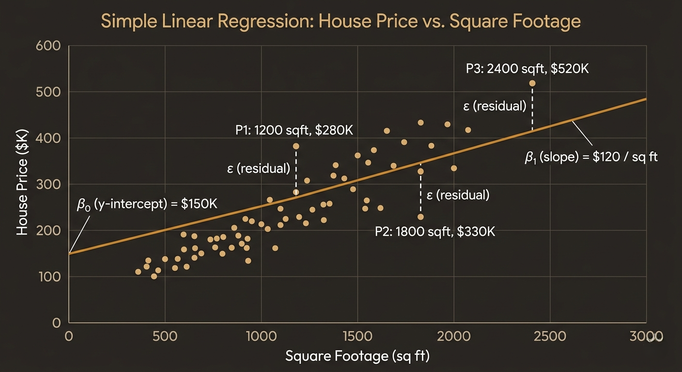
Simple linear regression finds the best straight-line relationship between two variables. The equation is foundational: ŷ = β₀ + β₁x + ε. Here, ŷ (pronounced "y-hat") is your prediction, x is your input feature, β₀ is where the line crosses the y-axis when x=0, and β₁ is the slope — how much ŷ changes for each unit increase in x. The ε (epsilon) is the residual: the gap between what your model predicts and what actually happened.

That residual is everything. It's not a nuisance to minimize and forget — it's diagnostic gold. The distribution, pattern, and scale of residuals tell you whether your model is correctly specified, whether it violates assumptions, and whether your predictions will generalize to new data. Most tutorials show you how to fit the line; this guide will show you how to interrogate it.

ŷ = β₀ + β₁x   |   residual ε = y − ŷ 💡 What Slope Actually Means

β₁ = 50 in a house-price model means: for every one additional square foot, the predicted price increases by $50. But this interpretation only holds if all other things are equal. In practice, square footage correlates with everything else (number of bedrooms, neighborhood quality, lot size). In simple regression, the slope absorbs the effects of everything you left out. This is why moving to multiple regression — while also more dangerous — is usually necessary for honest inference.

---

02OLS: How Your Computer Actually Finds the Best Line

Given n data points, there are infinitely many lines you could draw. What makes one "best"? Ordinary Least Squares (OLS) answers this with an elegant principle: choose the line that minimizes the sum of squared residuals. Square the vertical distance from each point to the line, add them all up, and minimize that total. The word "ordinary" distinguishes this from weighted or generalized least squares variants.

The reason we square residuals rather than taking absolute values is twofold. First, squaring penalizes large errors more heavily than small ones — if a prediction is off by 10, squaring gives 100 vs 100 from ten errors of magnitude 1. Second, squared functions are differentiable everywhere, which lets you find the exact minimum analytically by setting the derivative equal to zero. The normal equations give you closed-form solutions: β₁ = Σ(xᵢ − x̄)(yᵢ − ȳ) / Σ(xᵢ − x̄)².

For datasets that fit in memory, this analytical solution is exact and fast. But for very large datasets or when using regularization (Ridge, Lasso), you switch to gradient descent — an iterative optimization that updates β values step by step until convergence. This is why feature scaling matters for gradient descent but not for analytical OLS: the gradient descent step size is affected by feature magnitudes, while the normal equations aren't.

⚠️ When Analytical OLS Fails

If XᵀX is not invertible — which happens when you have perfect multicollinearity (one feature is a linear combination of others) or more features than observations — the normal equations have no unique solution. This is why Ridge regression adds a regularization term (λI) to make the matrix invertible. If you ever see sklearn throwing a "singular matrix" error or strange β values, this is probably why.

ols_from_scratch.py

import numpy as np

def ols_coefficients(X, y):
 """
 Solve for β using normal equations: β = (XᵀX)⁻¹Xᵀy
 X: feature matrix (n_samples, n_features)
 y: target vector (n_samples,)
 """
 # Add bias column (intercept β₀)
 X_b = np.column_stack([np.ones(len(X)), X])
 # Normal equations: (XᵀX)⁻¹ Xᵀy
 beta = np.linalg.inv(X_b.T @ X_b) @ X_b.T @ y
 return beta[0], beta[1:] # returns (β₀, [β₁, β₂, ...])

# Example: house size → price
sqft = np.array([800,1200,1600,2000,2400,3000])
price = np.array([150,220,290,360,420,510]) # $k

b0, b1 = ols_coefficients(sqft.reshape(-1,1), price)
print(ff"Intercept: ${b0[0]:.1f}k") # β₀
print(ff"Slope: ${b1[0]:.4f}k per sqft") # β₁
print(ff"Predicted price for 2200 sqft: ${(b0[0] + b1[0]*2200):.1f}k")

---

03Multiple Linear Regression: More Power, More Danger

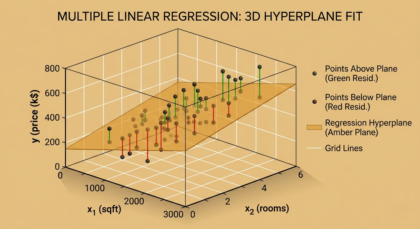
When you have more than one feature, simple linear regression becomes multiple linear regression (MLR). The equation extends naturally: ŷ = β₀ + β₁x₁ + β₂x₂ + ... + βₙxₙ + ε. Instead of a line in 2D space, you're fitting a hyperplane in (n+1)-dimensional space. The math works identically — OLS still minimizes the sum of squared residuals — but the interpretation of coefficients becomes more nuanced and the dangers multiply.

The most dangerous concept in MLR is multicollinearity: when two or more predictor variables are highly correlated with each other. Imagine predicting house prices using both square footage and number of rooms — these two variables are highly correlated (bigger houses generally have more rooms). The model struggles to separate the effect of each. It knows "size matters," but it can't reliably determine whether size's contribution comes from square footage or room count. The individual coefficients become unstable, sometimes swinging wildly with small changes to the dataset, even while the model's overall predictions remain reasonable.

Overfitting is the second major danger in MLR. Add enough features and your model memorizes the training data — achieving a near-perfect fit (R² → 1) but making terrible predictions on new data. The model has found patterns in the noise, not the signal. The fix: cross-validation, regularization (Ridge/Lasso), or simply being thoughtful about which features deserve to be in the model in the first place. Adding a feature should require justification; it doesn't come free.

ŷ = β₀ + β₁x₁ + β₂x₂ + ... + βₙxₙ 🔮 Myth: More Features = Better Model

The Variance-Bias tradeoff says: a model that's too simple underfits (high bias, can't capture the signal). A model that's too complex overfits (high variance, captures the noise). The sweet spot is a model that generalizes. Adding a feature reduces bias (less underfitting) but increases variance (more overfitting risk). The adjusted R² penalizes models for unnecessary features, unlike regular R² which always increases as you add more predictors — making regular R² dangerously misleading for model selection in MLR.

---

04Regression Metrics: Choosing the Right Scorecard

Here's the thing most tutorials miss: the choice of regression metric is not cosmetic. It changes what your model optimizes for, which errors it tolerates, and how you should interpret model performance. Using the wrong metric for your use case can lead you to select a model that looks great on paper but fails in production.

MAE (Mean Absolute Error) takes the average absolute difference between predictions and actuals. It's the most interpretable: if your model predicts house prices, an MAE of $15,000 means your predictions are off by $15K on average. MAE treats every dollar of error equally, making it robust to outliers. Its downside is that absolute value is not differentiable at zero, complicating some optimization scenarios.

MSE (Mean Squared Error) squares the errors before averaging. This means a $30K error counts for 4× as much as a $15K error — not twice as much. MSE punishes large errors disproportionately, making your model try harder to avoid catastrophic mistakes. The problem: MSE is in squared units (dollars squared), which is meaningless to stakeholders. RMSE (Root MSE) fixes this by taking the square root, returning to the original units. But RMSE still inherits MSE's outlier sensitivity.

R² (Coefficient of Determination) measures the proportion of variance in y that is explained by your model. An R² of 0.80 means 80% of the variation in house prices is captured by your features. R² = 1 is a perfect fit; R² = 0 means your model does no better than always predicting the mean. R² can be negative if your model is actively worse than the mean. Warning: R² always increases as you add features in MLR, regardless of whether those features are useful — use adjusted R² or cross-validated R² for model selection.

📏 Choosing Your Metric: Practical Guide

Use MAE when outliers are genuine extreme events that you want your model to handle gracefully (medical costs, ad revenues). Use RMSE when large errors are especially costly and you want to penalize them heavily (safety-critical predictions, batch manufacturing). Use R² for explaining model quality to non-technical stakeholders. Use adjusted R² for comparing models with different numbers of features. In production, always report multiple metrics — a model with great RMSE but terrible MAE often has a few catastrophically wrong predictions that deserve investigation.

regression_metrics.py

import numpy as np
from sklearn.metrics import mean_absolute_error, mean_squared_error, r2_score

y_true = np.array([220, 290, 360, 420, 510]) # actual prices ($k)
y_pred = np.array([215, 300, 355, 440, 500]) # predicted

mae = mean_absolute_error(y_true, y_pred)
mse = mean_squared_error(y_true, y_pred)
rmse = np.sqrt(mse)
r2 = r2_score(y_true, y_pred)

print(ff"MAE: ${mae:.1f}k (avg absolute error)")
print(ff"MSE: ${mse:.1f}k² (penalizes outliers heavily)")
print(ff"RMSE: ${rmse:.1f}k (same units as target)")
print(ff"R²: {r2:.3f} ({r2*100:.1f}% variance explained)")

# Adjusted R² (penalizes unnecessary features)
n, p = len(y_true), 1 # p = number of features
adj_r2 = 1 - (1-r2)*(n-1)/(n-p-1)
print(f"Adj R²: {adj_r2:.3f} (preferred for MLR model selection)")

---

05The LINE Assumptions: The Contract You're Signing

Every time you fit a linear regression model, you're implicitly signing a contract with four clauses. The acronym LINE covers them: Linearity, Independence, Normality of residuals, and Equal variance (Homoscedasticity). Violating these assumptions doesn't prevent you from getting a model — your software will happily produce coefficients no matter what. The problem is that your confidence intervals, p-values, and predictions become unreliable in ways that are hard to detect without deliberate diagnostics.

Linearity seems obvious but is routinely violated. You're assuming y is a linear function of x. If the true relationship is curved (e.g., diminishing returns on advertising spend), your linear model will systematically over-predict at extreme values and under-predict in the middle. The fix is usually feature engineering: add a squared term (x²), use a log transformation, or switch to a non-linear model.

Independence means that one observation's error doesn't predict another's. In time series data (stock prices, temperature readings, website traffic), consecutive observations are almost always correlated — yesterday's error tells you something about today's. This autocorrelation inflates your model's apparent precision, making it look more confident than it is. Normality of residuals is needed for valid hypothesis tests on coefficients — though with large samples, the Central Limit Theorem makes regression robust to this assumption. Homoscedasticity (equal variance) means the spread of residuals should be constant across all values of x. If residual spread increases with x (called heteroscedasticity), your standard errors are wrong.

⚠️ The Most Violated Assumption You Never Check

Independence is the assumption most people completely ignore, and its violation is the most damaging. If you're predicting monthly sales and your data includes multiple observations per customer, or multiple months for the same store, or any other repeated-measures structure — your observations are not independent, and your standard errors are almost certainly too small. This makes your coefficients look statistically significant when they're not. Always ask: "Is each row of my data truly a unique, independent observation?" If not, you need mixed-effects models or clustered standard errors.

assumption_checks.py

import numpy as np
import matplotlib.pyplot as plt
from scipy import stats
from sklearn.linear_model import LinearRegression

model = LinearRegression().fit(X_train, y_train)
residuals = y_train - model.predict(X_train)

# ── 1. Linearity: Residuals vs Fitted values ──────────────────
# No pattern should be visible — random scatter around y=0
fitted = model.predict(X_train)
plt.scatter(fitted, residuals, alpha=0.5)
plt.axhline(0, color='r', linestyle='--')
plt.title('Residuals vs Fitted — check for patterns')

# ── 2. Normality: Q-Q plot ─────────────────────────────────────
stats.probplot(residuals, dist="norm", plot=plt)

# ── 3. Homoscedasticity: Scale-location plot ──────────────────
plt.scatter(fitted, np.sqrt(np.abs(residuals)), alpha=0.5)
# Trend in this plot → heteroscedasticity problem

# ── 4. Independence: Durbin-Watson test ───────────────────────
from statsmodels.stats.stattools import durbin_watson
dw = durbin_watson(residuals)
print(ff"Durbin-Watson: {dw:.3f} (ideal ~2.0, <1.5 or>2.5 = autocorrelation)")

# ── 5. Multicollinearity: Variance Inflation Factor ───────────
from statsmodels.stats.outliers_influence import variance_inflation_factor
vif_data = {'feature': X.columns, 'VIF': [variance_inflation_factor(X.values, i) for i in range(X.shape[1])]}
# VIF > 10 indicates severe multicollinearity — act on it

---

06Residual Analysis: Reading the Model's Confessions

Residuals are where your model confesses everything it got wrong. A properly fitting linear regression produces residuals that look like white noise — no pattern, no trend, no clusters. When you see patterns in your residuals, your model is systematically wrong in ways that your input features aren't capturing. This is both a problem and an opportunity.

The four key diagnostic plots are: Residuals vs Fitted (checks linearity — should be random scatter around zero with no curve), Q-Q Plot (checks normality — residuals should fall on the diagonal line), Scale-Location Plot (checks homoscedasticity — the spread should be flat), and Residuals vs Leverage (identifies influential outliers — Cook's Distance > 1 warrants investigation).

Picture this: you fit a model predicting monthly website traffic and your residuals vs fitted plot shows a clear U-shape. This tells you the relationship is curved, not linear. Your model systematically under-predicts at low and high traffic levels (the bottom of the U) and over-predicts at medium levels. The fix: add a squared term (traffic²) or log-transform the target variable. The residual plot told you exactly what feature engineering to do.

✅ When Your Model Is "Good Enough"

Perfect diagnostics are a fantasy in real data. The question is always "are the violations severe enough to invalidate my conclusions?" Minor heteroscedasticity with large samples? Often fine. Mild non-normality with n > 100? The CLT protects your inference. Severe multicollinearity? Usually not fine — your coefficient estimates are garbage even if predictions look okay. Clear non-linearity in residuals? Not fine — you're systematically biased. Calibrate your diagnostic worry to the severity of violation and the stakes of your decision.

---

synthesisHow It All Connects: The Complete Linear Regression Workflow

Linear regression is not just an algorithm — it's a workflow. You start with data and a question. You fit a simple model, check residuals for violations, transform features or add terms to address them, re-fit. You select the right metric (MAE, RMSE, R²) based on your use case and audience. You check the LINE assumptions, use adjusted R² and cross-validation for model selection, and finally check multicollinearity via VIF before reporting coefficients as meaningful estimates.

Every piece connects: OLS minimizes MSE (that's the loss function), making RMSE the natural evaluation metric. The LINE assumptions are the conditions under which OLS gives you the Best Linear Unbiased Estimators (the Gauss-Markov theorem). Residual analysis checks those assumptions diagnostically. Multiple regression extends the math but introduces multicollinearity and overfitting as new failure modes. The tools — VIF, adjusted R², cross-validation — are the defenses against those failure modes.

---

07Getting Started: Production-Ready Linear Regression in Python

complete_pipeline.py

from sklearn.datasets import fetch_california_housing
from sklearn.model_selection import train_test_split, cross_val_score
from sklearn.preprocessing import StandardScaler
from sklearn.linear_model import LinearRegression
from sklearn.metrics import mean_absolute_error, mean_squared_error, r2_score
from sklearn.pipeline import Pipeline
import numpy as np
import pandas as pd

# ── 1. Load data ──────────────────────────────────────────────
data = fetch_california_housing(as_frame=True)
X, y = data.frame.drop('MedHouseVal', axis=1), data.frame['MedHouseVal']

# ── 2. Split ──────────────────────────────────────────────────
X_tr, X_te, y_tr, y_te = train_test_split(X, y, test_size=0.2, random_state=42)

# ── 3. Pipeline: scale → fit ─────────────────────────────────
pipe = Pipeline([('scaler', StandardScaler()), ('lr', LinearRegression())])

# ── 4. Cross-validate ────────────────────────────────────────
cv_rmse = np.sqrt(-cross_val_score(pipe, X_tr, y_tr, cv=5, scoring='neg_mean_squared_error'))
print(ff"CV RMSE: {cv_rmse.mean():.3f} ± {cv_rmse.std():.3f}")

# ── 5. Final evaluation ────────────────────────────────────── 
pipe.fit(X_tr, y_tr)
y_pred = pipe.predict(X_te)
print(ff"Test MAE: {mean_absolute_error(y_te, y_pred):.3f}")
print(ff"Test RMSE: {np.sqrt(mean_squared_error(y_te, y_pred)):.3f}")
print(ff"Test R²: {r2_score(y_te, y_pred):.3f}")

# ── 6. Coefficient table ──────────────────────────────────────
lr = pipe.named_steps['lr']
coef_df = pd.DataFrame({'Feature': X.columns, 'Coefficient': lr.coef_})
print(coef_df.sort_values('Coefficient', ascending=False))

FAQFrequently Asked Questions

What is the difference between linear regression and logistic regression? + Linear regression predicts a continuous target value (price, temperature, sales volume). Logistic regression predicts the probability of a categorical outcome (yes/no, spam/not spam) by passing a linear combination through a sigmoid function to squash output to [0,1]. The name "logistic regression" is misleading — it's actually a classification algorithm despite having "regression" in its name. You use linear regression for continuous targets and logistic regression (or other classifiers) for categorical ones. Using linear regression for binary classification is technically possible but produces probabilities outside [0,1] and violates homoscedasticity assumptions. When should I use MAE vs RMSE? + Use MAE when you want outliers to count proportionally to their error (robust to extreme values), and when the average error magnitude is more interpretable to your audience than a squared average. MAE is the right choice when large errors and small errors should be treated symmetrically — a $50K prediction error is exactly 10× worse than a $5K error. Use RMSE when large errors are disproportionately costly — a $50K error should be penalized more than 10× a $5K error. RMSE is also preferred when your optimization objective (the loss function) is MSE, making RMSE directly comparable to training loss. In practice, always report both. Can R² be negative? What does that mean? + Yes. R² = 1 − (SS_residuals / SS_total), where SS_total is the total sum of squared deviations from the mean. If your model's residuals are larger than the total variance (i.e., your model is worse than just predicting the mean for every observation), then SS_residuals > SS_total and R² becomes negative. This typically happens when you make a serious modeling mistake: using a model trained on one dataset to predict a completely different one, or using a non-intercept model that forces the line through the origin. A negative R² is a red flag, not a mathematical impossibility. What is multicollinearity and how do I detect and fix it? + Multicollinearity occurs when two or more predictor variables are highly correlated. Detection: compute Variance Inflation Factor (VIF) for each feature. VIF > 5 is concerning, VIF > 10 is severe. You can also look at the correlation matrix — any pair above ~0.8 correlation deserves scrutiny. Fixes in order of invasiveness: (1) Drop one of the correlated features if they represent similar information. (2) Combine them into a single feature (e.g., average). (3) Use Ridge Regression, which adds regularization that stabilizes coefficient estimates under collinearity. (4) Use PCA to transform correlated features into uncorrelated principal components. Note: multicollinearity doesn't affect predictions if you only need the model for forecasting — it only corrupts the interpretation of individual coefficients. What is homoscedasticity and why does it matter? + Homoscedasticity means "equal spread" — the variance of residuals should be constant across all fitted values. Heteroscedasticity (unequal spread) is the violation. In a house price model, you might find that predictions for cheap houses are off by ±$10K but predictions for expensive houses are off by ±$100K — the residuals grow with house price. This violates the assumption. Why it matters: OLS standard errors assume constant variance. With heteroscedasticity, standard errors are wrong, making hypothesis tests and confidence intervals unreliable. Fixes: use weighted least squares (WLS), transform the target variable (log-price often helps), or use heteroscedasticity-consistent (HC) standard errors in your inference. How is adjusted R² different from regular R², and when should I use it? + Regular R² always increases (or stays the same) when you add more features, even if those features are completely random noise. This makes it useless for comparing models with different numbers of predictors. Adjusted R² penalizes model complexity: Adj R² = 1 − (1−R²)(n−1)/(n−p−1), where n is sample size and p is number of predictors. Adding a weak feature can actually decrease adjusted R² while increasing regular R². Always use adjusted R² (or cross-validated R²) when comparing models with different feature counts. For reporting to non-technical stakeholders, regular R² is fine, but note that it's for the specific model you chose — it's not directly comparable to alternative specifications. What is the difference between Ridge and Lasso regression? + Both are regularized versions of linear regression that add a penalty term to the loss function to prevent overfitting. Ridge (L2) adds λ × Σβᵢ² to the loss, shrinking all coefficients toward zero but never to exactly zero — it handles multicollinearity well. Lasso (L1) adds λ × Σ|βᵢ|, which can shrink some coefficients to exactly zero, effectively performing feature selection. Use Ridge when you believe all features are relevant but multicollinearity is causing instability. Use Lasso when you suspect many features are irrelevant and want the model to select a sparse subset automatically. Elastic Net combines both penalties and is often a practical compromise. Does linear regression require feature scaling? + For analytical OLS (the normal equations), no — the math produces identical predictions regardless of feature scale. But there are important practical reasons to scale: (1) Gradient descent converges much faster with scaled features — without scaling, the cost function is elongated and descent is slow and oscillatory. (2) Ridge and Lasso regularization apply equal penalty to all coefficients by default, so unscaled features with larger magnitudes effectively receive less regularization — leading to unfair penalization. (3) Comparing coefficient magnitudes to gauge feature importance only makes sense on standardized features. As a best practice, always scale before fitting any regularized model or when using gradient-based optimization.

📈 Regression Lab

Four interactive experiments — drag points, compare metrics, diagnose residuals, and explore multicollinearity.

Click to add points · Drag existing points · Amber line = OLS fit · Dashed = your manual guess

OLS Line Fitter

Click the canvas to add data points. The amber line shows the OLS best fit — it minimizes the sum of squared residuals automatically.

Manual slope (β₁) 0.00 Manual intercept (β₀) 0.00 — OLS β₀ (intercept) — OLS β₁ (slope) — R² score — Manual SSE OLS: SSE = — Manual: SSE = — OLS always wins ↑

Error distribution — actual vs predicted with residuals shown

Regression Metrics Explorer Prediction error level Medium Outlier severity None — MAE — MSE — RMSE — R²

Residuals vs Fitted values — look for patterns

Normal Q-Q plot — points should fall on the line

LINE Assumptions Diagnostics Violation Type Violation severity 50% — R² — RMSE — Linearity — Homoscedasticity

Coefficient stability under multicollinearity — watch β₁ and β₂ become unreliable

Multicollinearity Explorer Correlation ρ(x₁,x₂) 0.00 Sample size 100 — VIF (x₁) — β₁ std dev — β₂ std dev — Model R²

Key insight: As ρ → ±1, the VIF explodes and the distribution of β estimates widens dramatically. R² stays high — predictions remain good — but individual coefficients become meaningless.