How Diffusion Models Work: The Physics Behind AI Image & Video Generation

Diffusion Models — Physics & AI · 3,800 words · 4 interactive labs · April 2026

How Diffusion Models Work:
The Physics Behind AI Image & Video Generation

DALL·E, Stable Diffusion, Sora, and WAN 2.1 all share the same stunning secret: they're running Brownian motion in reverse, in billion-dimensional space. Here's the complete story — with interactive simulations you can run right now.

Read the Deep Dive ↓ Open Physics Lab 🌀 Table of Contents

1. Brownian Motion & the Physics Connection
2. CLIP: The Shared Language of Images and Words
3. DDPM: Why Naive Denoising Fails
4. Vector Fields & Score Functions
5. DDIM: Deterministic Generation
6. Classifier-Free Guidance
7. Negative Prompts & Steering
8. Getting Started: Run WAN 2.1

01Brownian Motion Run Backwards: The Wildest Idea in Modern AI

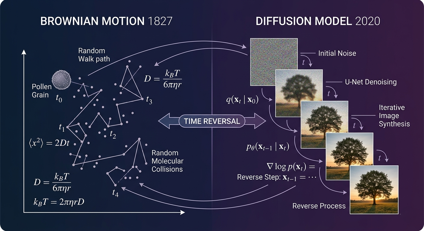
In 1827, botanist Robert Brown was staring at pollen grains suspended in water under a microscope when he noticed something strange: they moved. Not because they were alive, but because invisible water molecules were constantly bombarding them from all sides, pushing them in random, jerky paths. This phenomenon — Brownian motion — became one of the cornerstone validations of atomic theory when Einstein described it mathematically in 1905.

One hundred and fifteen years later, a team of researchers at UC Berkeley made one of the most counterintuitive connections in computer science history: generating photorealistic images is mathematically equivalent to running Brownian motion backwards, in a space with millions of dimensions. This isn't a metaphor or a loose analogy. The differential equations governing how pollen grains diffuse through water are the same equations, with time reversed, that govern how a diffusion model turns noise into a photograph.

Here's why this matters practically. When you generate an image with DALL·E or Stable Diffusion, the process begins by sampling pure Gaussian noise — a video or image where every pixel value is chosen independently at random. This noise is then fed through a neural network, step by step, with each step making the image slightly less noisy and slightly more structured. The physics connection gives us real algorithms — not just intuition — for how to run this process efficiently, how many steps to take, and crucially, whether to add randomness during generation or not.

💡 The Physics Analogy Is Literal, Not Metaphorical

Diffusion models were named after the physical diffusion process for a precise mathematical reason. The forward process (adding noise to images step by step) follows a stochastic differential equation identical to the Langevin equation describing Brownian motion. The generative process (turning noise back into images) exploits the time-reversal symmetry of this equation — a property proven in statistical mechanics. This connection gives us the Fokker-Planck equation, which is what enabled DDIM's breakthrough.

---

02CLIP: Learning the Shared Geometry of Words and Pictures

Before images can be steered by text prompts, something remarkable has to happen: language and pixels have to be mapped into the same geometric space so that "a photo of a cat" and an actual photograph of a cat point in similar directions in a high-dimensional vector space. This is what CLIP — Contrastive Language-Image Pre-training — accomplishes, and it's one of the most elegant training objectives in machine learning.

CLIP is composed of two separate encoder networks: one for images, one for text. Both produce 512-dimensional vectors. The training objective is beautifully simple to state: given a batch of image-caption pairs, make the vector for each image close to the vector for its corresponding caption, while simultaneously pushing vectors for non-matching pairs apart. This "contrastive" training — rewarding alignment of matching pairs and penalizing alignment of mismatched pairs — is applied across the full batch simultaneously. With 400 million training pairs from the internet, the result is a shared embedding space where semantic meaning has a real geometric structure.

The properties of this learned space are remarkable. Take two photos of the same person — one with a hat and one without. The difference vector (hat photo − no-hat photo) corresponds, when searched against all text embeddings, to the word "hat." This isn't hardcoded; it emerged from training. The model has learned that the direction "add hat to a person" is a distinct, identifiable direction in this space. DALL·E 2's creative name, unCLIP, refers to inverting this — taking a point in CLIP's text embedding space and generating the image that lives there.

⚠️ CLIP Embeddings Only Go One Direction

CLIP solves a representation problem, not a generation problem. It can map images and text into a shared space, but it can't go the other way — you can't give it an embedding vector and get a photo back. This is why diffusion models were needed: they solve the inverse mapping, generating images that correspond to a given embedding. CLIP provides the "what we want" direction; diffusion models do the "how to get there" computation.

clip_similarity.py

import torch
from transformers import CLIPModel, CLIPProcessor

model = CLIPModel.from_pretrained("openai/clip-vit-base-patch32")
processor = CLIPProcessor.from_pretrained("openai/clip-vit-base-patch32")

# Compare text candidates to an image using cosine similarity
texts = ["a photo of a cat", "a photo of a dog",
 "a landscape painting", "a person wearing a hat"]

inputs = processor(text=texts, images=image,
 return_tensors="pt", padding=True)
with torch.no_grad():
 outputs = model(**inputs)
 logit_per_image = outputs.logits_per_image
 probs = logit_per_image.softmax(dim=1) # cosine sim → probabilities

for text, prob in zip(texts, probs[0]):
 print(f"{text:35s}: {prob.item():.4f}")
# → a photo of a cat : 0.9812 ← correct!

---

03DDPM: Why the Naive Approach to Diffusion Doesn't Work

In June 2020, a team at UC Berkeley published "Denoising Diffusion Probabilistic Models" (DDPM), the paper that put diffusion on the map as a viable image generation approach. The core idea seems straightforward enough: add noise to images step by step until they're destroyed, then train a neural network to reverse this process. But the specific training and generation algorithms they arrived at contain two surprises that most introductory explanations completely miss.

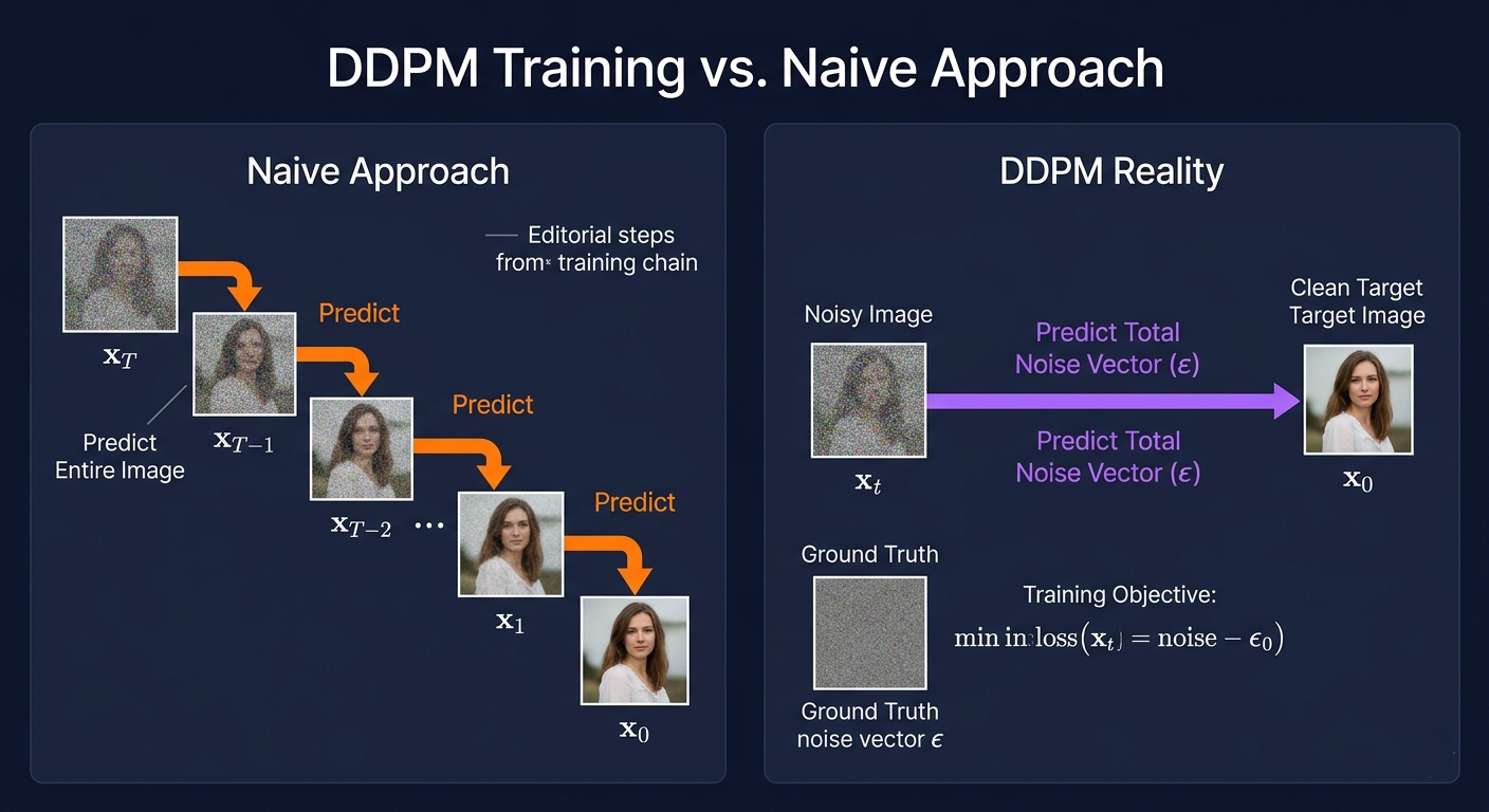
Surprise one: the training objective isn't what you'd expect. The naive approach would be to train the model to denoise images one step at a time — take step 100's noisy image, predict step 99's slightly-less-noisy version. Instead, the Berkeley team trained their model to predict the total noise added to the original clean image across all steps simultaneously. Rather than asking "what is the previous step?", they ask "what is the entire noise vector from clean to here?" This seems harder, but it dramatically reduces training variance because the model's target is a single consistent vector rather than a noisy intermediate.

Surprise two: during image generation, the algorithm deliberately adds fresh random noise at every step — even though you're trying to remove noise. This seems backwards. If you're trying to denoise, why keep adding noise? The answer, as we'll see in the vector field section, is that without this added noise, all generated images collapse toward the average of the training distribution. Adding noise is what preserves diversity and produces sharp, specific images rather than blurry averages.

🔮 Myth: Diffusion Models Denoise One Step at a Time

This is the most common misconception about how diffusion models work. Modern diffusion models do not predict "image at step N-1 given image at step N." They predict the total noise vector added across all steps — effectively pointing from the current position all the way back to the original clean image. This choice, combined with the time-conditioning trick, is the key insight that made diffusion models work in practice. The naive step-by-step approach produces poor results.

ddpm_forward.py

import torch
import numpy as np

# DDPM forward process: add noise to image at timestep t
def add_noise(x0, t, noise=None, T=1000):
 """
 x0: clean image
 t: timestep (0 = clean, T = pure noise)
 Returns: noisy image at timestep t
 """
 if noise is None:
 noise = torch.randn_like(x0)
 # Linear beta schedule (simplified)
 beta_min, beta_max = 0.0001, 0.02
 betas = torch.linspace(beta_min, beta_max, T)
 alphas = 1.0 - betas
 alphas_cumprod = torch.cumprod(alphas, dim=0)
 sqrt_alpha = alphas_cumprod[t] ** 0.5
 sqrt_1m_alpha = (1 - alphas_cumprod[t]) ** 0.5
 # The DDPM magic: closed-form noise at any timestep
 xt = sqrt_alpha * x0 + sqrt_1m_alpha * noise
 return xt, noise # return noisy image AND the noise (training target!)

# The model is trained to predict 'noise' given (xt, t)
# NOT to predict x_{t-1} given xt — that's the common misconception

---

04Vector Fields & Score Functions: The Geometric Heart of Diffusion

The cleanest way to understand what diffusion models are actually learning is to think geometrically. Imagine your training images as points scattered in a very high-dimensional space — each pixel's intensity value is one coordinate, so a 512×512 image lives in a space with 786,432 dimensions. The set of all realistic images forms a thin, complex manifold in this space. A diffusion model's job is to learn a vector field — an arrow at every point in this space — that points toward the manifold of realistic images.

This is easiest to visualize in 2D. Imagine your training data forms a spiral. Every point in the 2D plane gets an arrow pointing toward the nearest part of the spiral. Starting from random noise (a random point in the plane), you follow these arrows step by step until you land on the spiral. That's image generation. The diffusion model doesn't memorize images — it learns the vector field of arrows pointing toward realistic-image-land.

The time conditioning is what makes this work. At early steps (high noise, far from the spiral), the vector field points coarsely toward the general center of mass of the data. As you get closer (lower noise, closer to the spiral), the vector field becomes more refined, pointing toward the specific local structure. Without time conditioning, a single vector field couldn't handle both the coarse long-range guidance and the fine local structure. This time-varying vector field is also known as the score function — the gradient of the log-probability of the data distribution — which connects diffusion models deeply to score-based generative modeling.

🌀 The Phase Transition Moment

Researchers have observed something striking when watching the vector field evolve as time decreases toward zero: there appears to be a phase transition. The arrows initially point toward the center of the data distribution, and then — at a specific value of t — they suddenly reorient to point toward the detailed local structure. This is analogous to a physical phase transition (like water freezing). Understanding and controlling this transition point is an active area of research for improving generation quality and speed.

score_function.py

import torch

# The score function ∇_x log p(x) points toward higher-density regions
# Diffusion models learn to approximate this

def score_function_estimate(model, x, t):
 """
 Given a noisy sample x at timestep t,
 our model predicts the noise ε that was added.
 We can convert this to a score function estimate.
 """
 pred_noise = model(x, t) # model predicts ε
 sigma_t = get_sigma(t) # noise scale at time t
 # Score function ≈ -ε/σ_t (negative predicted noise / noise scale)
 # This vector points TOWARD the data manifold
 return -pred_noise / sigma_t

# Key insight: the model learns the score function, NOT a direct image predictor
# The score is a vector field — arrows pointing toward realistic images
# More noise (large t) → coarse arrows → less noise (small t) → fine arrows

---

05DDIM: Generating Images Without Any Randomness

The DDPM algorithm required adding random noise at every generation step. This kept images diverse and prevented the "blurry average" problem, but it also meant needing many steps (typically 1000) to generate high-quality images — each step requiring a full forward pass through a large neural network. At inference time, this was brutally slow.

Here's the thing most tutorials miss about DDIM: the key insight came from physics, specifically from the Fokker-Planck equation in statistical mechanics. The DDPM generation process is governed by a stochastic differential equation — a differential equation with both deterministic and random components. The Fokker-Planck equation tells us that for any stochastic differential equation governing the evolution of a probability distribution, there exists an equivalent ordinary differential equation — purely deterministic, no randomness — that produces the exact same final probability distribution.

This is what DDIM exploits. By switching from the stochastic DDPM update to the deterministic ODE-based update, generation becomes completely reproducible (same initial noise → same output every time), and the step sizes can be dramatically adjusted to skip steps. DDPM needed ~1000 steps. DDIM can produce excellent results in 20-50 steps, a 20-50× speedup with no changes to the trained model. The WAN video generation model uses an even more general version of this idea called flow matching, which parameterizes the ODE differently for further efficiency gains.

✅ DDIM: Same Model, Radically Different Sampling

The remarkable thing about DDIM is that it requires zero changes to model training. You train a diffusion model with the standard DDPM objective, and then at inference time you simply change the sampling algorithm from stochastic DDPM to deterministic DDIM. The final distribution of generated images is guaranteed (by the Fokker-Planck theory) to be the same. This means any pre-trained diffusion model can immediately benefit from DDIM sampling — which is why virtually all modern image generators use it or a variant of it.

ddim_sampling.py

import torch

def ddim_step(model, x_t, t, t_prev, eta=0.0):
 """
 DDIM sampling step (deterministic when eta=0)
 eta=0: DDIM (fully deterministic, fast)
 eta=1: DDPM (stochastic, slower but sometimes sharper)
 """
 pred_noise = model(x_t, t) # predict noise ε
 alpha_t = get_alpha(t)
 alpha_t_prev = get_alpha(t_prev)

 # Predict x0 directly from current noisy image
 x0_pred = (x_t - ((1-alpha_t)**0.5) * pred_noise) / (alpha_t**0.5)

 # DDIM deterministic update (no random noise when eta=0)
 sigma = eta * ((1-alpha_t_prev) / (1-alpha_t)) ** 0.5 * \
 ((1-alpha_t/alpha_t_prev)) ** 0.5

 noise = torch.randn_like(x_t) if eta > 0 else 0
 x_prev = (alpha_t_prev**0.5) * x0_pred + \
 ((1-alpha_t_prev-sigma**2)**0.5) * pred_noise + sigma * noise
 return x_prev # clean enough to use with 20 steps instead of 1000!

---

06Classifier-Free Guidance: The Trick That Makes Prompts Work

Conditioning a diffusion model on text seems straightforward: just pass the CLIP text embedding as an additional input to the denoising network, along with the noisy image and the timestep. The model should learn to use this text information to produce images that match the prompt. In practice, this works — but poorly. A model trained only with conditioning often fails to follow the prompt closely, getting distracted by the learned prior over all images.

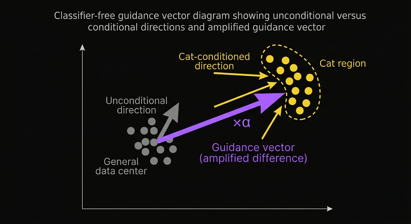
The insight behind classifier-free guidance is to train two models simultaneously: one that uses text conditioning (conditioned model), and one that doesn't (unconditional model). In practice, this is done with a single model by randomly zeroing out the text input during training for some fraction of examples. At generation time, you run both: the conditioned model gives you the direction toward your specific prompt, and the unconditional model gives you the general "this looks realistic" direction. The difference between these two — conditioned vector minus unconditional vector — is a vector pointing specifically toward your prompt, stripped of the general "be realistic" component.

You then amplify this difference by a scaling factor α (the guidance scale) and add it to the unconditional direction. With α=1, you get pure conditioning. With α=7 or α=15 (common defaults in Stable Diffusion), the model is strongly pushed toward the prompt, often producing more vibrant, detailed, and prompt-adherent images — at the cost of slightly less photorealistic diversity. This guidance scale is the "creativity vs accuracy" dial you see in every image generation interface, and understanding it as a geometric amplification makes the tradeoff immediately intuitive.

⚠️ Higher Guidance Scale ≠ Always Better

Beyond a certain guidance scale (typically around 10-15 for most models), image quality actually degrades. The geometric interpretation explains why: you're amplifying the difference between the conditioned and unconditioned vector fields so aggressively that the resulting direction overshoots the natural manifold of realistic images. Images look over-saturated, with artifacts and anatomical distortions. Most production systems cap guidance scale around 7.5 for this reason. Always test; the right value is prompt-dependent.

cfg_sampling.py

def classifier_free_guidance_step(model, x_t, t, text_emb,
 guidance_scale=7.5):
 """
 Classifier-Free Guidance (CFG) sampling step.
 Amplifies the difference between conditional and unconditional predictions.
 """
 # Unconditional: no text prompt (empty string embedding)
 null_emb = get_null_embedding()
 noise_uncond = model(x_t, t, null_emb) # ε_uncond

 # Conditional: with our text prompt
 noise_cond = model(x_t, t, text_emb) # ε_cond

 # CFG: amplify the "prompt-specific" direction
 # w=1: pure conditional, w>1: exaggerate prompt adherence
 noise_guided = (noise_uncond
 + guidance_scale * (noise_cond - noise_uncond))

 # More geometric: guidance_scale amplifies the "prompt direction"
 # guidance_scale=7.5 means: 7.5× amplification of prompt signal
 # Too high (>12) → artifacts, oversaturation, distortion
 return ddim_step(model, x_t, t, t_prev, noise_guided)

---

07Negative Prompts: Steering Away From What You Don't Want

Standard classifier-free guidance subtracts an unconditioned direction (empty prompt) from the conditioned direction. Negative prompts take this further: instead of subtracting a null embedding, you subtract the embedding of a description of what you explicitly don't want. If you want a realistic astronaut video, you subtract the embedding of "blurry, low quality, cartoonish, extra fingers, walking backwards" — and the resulting guidance vector points even more strongly toward your positive prompt and away from these failure modes.

The WAN 2.1 video generation model's default negative prompt is a fascinating window into what these models tend to produce without guidance. It includes obvious quality issues (blurry, pixelated, watermark) but also revealing behavioral artifacts: "extra fingers" (the classic AI hand failure), "walking backwards," and — intriguingly — the entire prompt is written in Chinese, suggesting the model was trained on a multilingual corpus where Chinese-language quality signals were particularly strong. This is a perfect illustration of how negative prompts encode learned knowledge about model failure modes.

The geometric interpretation is clean: your positive prompt defines the direction you're amplifying toward. Your negative prompt defines a direction you're amplifying away from. The final guidance vector is the combination. You can think of positive and negative prompts as defining a subspace in the CLIP embedding space, and CFG as projecting your generation trajectory onto the most prompt-relevant component of this subspace — while simultaneously rejecting the negative-prompt component.

💡 Negative Prompts as Model Behavior Documentation

Reading a model's default negative prompt tells you more about its failure modes than any benchmark. WAN 2.1's inclusion of "walking backwards" tells you the model has a tendency to generate reversed motion — likely from training on videos where frame order ambiguity is common. "Extra fingers" tells you spatial consistency is a known weakness. If you're evaluating a new model for production, inspect its recommended negative prompt closely. It's the team's own documentation of what the model does without correction.

---

synthesisHow It All Connects: From Physics to Photorealism

The architecture of modern AI image and video generation is a stack of elegant ideas that happen to fit together almost too perfectly. CLIP learns a shared geometric space where text and images are comparable vectors. DDPM shows that you can learn to generate images by learning to reverse Brownian motion in this space. The score function interpretation shows that what's being learned is a vector field pointing toward realistic images. DDIM shows that this vector field can be traversed deterministically, dramatically reducing compute. And classifier-free guidance shows that the difference between the conditioned and unconditioned vector fields encodes the precise direction of your prompt — which can be amplified to control generation fidelity.

The fact that these pieces fit together is genuinely remarkable. The physics connection isn't decorative — it provides real algorithms. The CLIP embedding isn't just for classification — it becomes the steering wheel for generation. The randomness in DDPM isn't a bug — it's the mathematical requirement for sampling from a distribution rather than predicting its mean. Each design choice connects to the others through consistent mathematical reasoning.

---

08Getting Started: Run WAN 2.1 Locally

WAN 2.1 is the open-source model showcased in the video. Here's how to run it locally and experiment with everything we've covered — prompts, negative prompts, guidance scale, and step count.

wan_quickstart.sh

# Step 1: Install dependencies (requires Python 3.10+, CUDA GPU recommended)
pip install torch torchvision transformers diffusers accelerate

# Step 2: Install WAN 2.1 via diffusers
# WAN 2.1 model: Wan-AI/Wan2.1-T2V-1.3B (smaller) or 14B (larger)

# Step 3: Generate a video with Python

generate_video.py

import torch
from diffusers import AutoPipelineForText2Video

pipe = AutoPipelineForText2Video.from_pretrained(
 "Wan-AI/Wan2.1-T2V-1.3B",
 torch_dtype=torch.bfloat16,
 device_map="auto"
)

positive_prompt = """
An astronaut floating in space, holding an American flag.
Photorealistic, 4K, dramatic lighting, cinematic.
"""

negative_prompt = """
低质量, 模糊, 卡通, 多余的手指, 向后走
""" # WAN's default negative prompt — in Chinese!

video = pipe(
 prompt=positive_prompt,
 negative_prompt=negative_prompt,
 num_inference_steps=50, # DDIM steps (try 20 for faster)
 guidance_scale=6.0, # CFG scale (higher → more prompt-adherent)
 num_frames=81, # ~3 seconds at 24fps
 height=480, width=832,
).frames[0]

# Save as MP4
from diffusers.utils import export_to_video
export_to_video(video, "astronaut.mp4", fps=24)
print("Generated! Open astronaut.mp4")

FAQFrequently Asked Questions

What's the difference between DALL·E, Stable Diffusion, and Midjourney? + All three use diffusion models at their core, but differ in implementation and training. DALL·E 2/3 (OpenAI): closed-source, DALL·E 2 used the unCLIP approach (inverting CLIP embeddings), DALL·E 3 trains a captioner to improve prompt adherence. Stable Diffusion: open-source, operates in a compressed "latent space" (Latent Diffusion Models) rather than pixel space, making it faster. Midjourney: closed-source, trained with significant human preference feedback to produce aesthetically pleasing outputs. The core diffusion algorithm and DDIM sampling are shared across all three; the differences are training data, conditioning approaches, and fine-tuning strategies. What is latent diffusion and how does it differ from pixel-space diffusion? + Pixel-space diffusion operates directly on image pixels — for a 512×512 image, the model processes 786,432-dimensional vectors at each step. This is computationally expensive. Latent diffusion (used in Stable Diffusion) first compresses images using an autoencoder (VAE) into a much smaller "latent" representation (typically 64×64×4), runs diffusion in this compressed space, and then decodes the final latent back to pixels. The diffusion model only needs to process ~16,384 numbers per step instead of 786,432 — an ~50× reduction in dimensionality that makes the model dramatically faster while retaining most image quality. Why does adding random noise during generation improve image quality? + Because diffusion models learn to predict the mean (average) of the distribution at each step, not to directly sample from it. Without added noise, all generated images converge toward the mean of the training distribution, which looks blurry and generic. Adding Gaussian noise at each step is the mathematical mechanism for actually sampling from the full distribution rather than predicting its center. DDIM solves this differently by using a modified step size that keeps trajectories on the correct distribution contours without randomness — essentially following the ODE formulation that the Fokker-Planck equation guarantees produces the same distribution. What is flow matching and how does it relate to DDIM? + Flow matching is a generalization of the diffusion framework that directly parameterizes the ODE connecting noise to data using simpler, straighter trajectories. In DDPM/DDIM, the paths from noise to image follow complex curved trajectories in embedding space because of the Gaussian noise schedule. Flow matching uses linear interpolation paths from noise to data, which are easier for the model to learn and require fewer steps at inference time. WAN 2.1 uses flow matching, which is why it can produce high-quality video with fewer DDIM steps than equivalent DDPM-based models. Meta's Movie Gen and many recent state-of-the-art video models also use flow matching. What does "guidance scale" actually control, geometrically? + Guidance scale (α) amplifies the component of the denoising direction that is specific to your prompt, after removing the general "be realistic" direction. Geometrically: conditioned vector − unconditioned vector = "prompt-specific" direction. Multiplying this by α and adding to the unconditioned direction gives the final guidance vector. With α=1: pure conditioning, like the model just seeing your prompt. With α=7: 7× amplification of the prompt-specific signal. With α=0: identical to unconditioned generation, your prompt has no effect. Beyond α≈12 for most models: the direction overshoots the manifold of realistic images, causing artifacts and incoherence. Can diffusion models run on consumer hardware? + Yes, with the right model. Stable Diffusion 1.5 and SDXL run on consumer GPUs with 8GB+ VRAM. With quantization (4-bit or 8-bit), even smaller GPUs work. For video, WAN 2.1's 1.3B parameter model requires ~6GB VRAM; the 14B model needs ~40GB (typically multi-GPU). CPU generation is possible but extremely slow. Tools like ComfyUI, Automatic1111, and InvokeAI provide user-friendly interfaces. The key optimization is latent diffusion — running in compressed space — which is what makes consumer hardware viable at all. Flux (Black Forest Labs) is another high-quality open model that's become popular for consumer hardware in 2024-2025. What is ControlNet and how does it extend guidance? + ControlNet extends conditional generation by adding spatial structure conditioning on top of text. Instead of just a text embedding, you can provide edge maps, depth maps, pose skeletons, or reference images as additional conditioning signals. A small adapter network processes these spatial conditions and injects them into the diffusion model via additional cross-attention connections. This allows precise control over composition, pose, and structure while still using natural language for style and content. ControlNet is the technique behind "consistent character" generation, architectural visualization from floor plans, and pose-controlled image generation. Why do AI-generated images still struggle with hands? + Hands are geometrically complex, highly variable, and appear in many orientations — making them one of the hardest structural elements to model. More importantly, the high-dimensional space of realistic images has a complex manifold for hands specifically: the number of fingers, their joints, and their spatial relationships form a highly constrained submanifold. Diffusion models operating in this space can end up at points that look globally realistic but locally violate the anatomical constraints of hands. Newer models trained with more hand-specific data and longer training have significantly improved (GPT-4o's image generation and FLUX are much better than SD1.5), but perfect hands remain an active research challenge, partly because the negative prompt "extra fingers" has become a crutch rather than a solution.

🌀 Physics Lab

Four interactive experiments spanning Brownian motion, CLIP embedding space, diffusion vector fields, and classifier-free guidance.

Forward diffusion (adding noise) ↔ Reverse diffusion (generating images) — click to place starting point

Brownian Motion / Diffusion Lab Number of Particles 50 Noise Scale (σ) 0.02 Data Distribution Direction 0 Step — Spread (σ) 50 Particles Forward Direction

Try: Run Forward until particles are pure noise. Switch to Reverse and watch them collapse back toward the data distribution. This is exactly what AI image generators do — in 786,432 dimensions.

2D projection of CLIP embedding space — hover to see cosine similarity · click to select

CLIP Embedding Explorer Image Concept Arithmetic Operation Nearest Text Neighbors 512 Dimensions — Top Match — Cosine Similarity None Operation

Learned vector field — arrows point toward data manifold · darker = high t, brighter = low t

Generation trajectories — with noise (DDPM) vs without (deterministic)

Vector Field Configuration Time t 0.50 Num Particles 20 Noise (η) DDPM 0 Steps — On Manifold — Diversity DDPM Algorithm

Guidance vector visualization — gray=unconditioned, yellow=conditioned, violet=guided

Classifier-Free Guidance Simulator Guidance Scale (α) 7.5 Target Class Negative Prompt Guidance Analysis Click Run to analyze guidance vectors... 7.5 Guidance Scale — Amplification — Class Coverage — Quality Est.

Try: Set guidance to 0 (unconditioned — any random image). Raise to 7.5 (good balance). Go to 20+ and watch quality estimates drop — the "overshoot" problem.