Gradient Descent Explained: The Algorithm That Trains Every AI Model

Optimization Engine of Deep Learning · 3,900 words · 4 interactive labs · April 2026

θ_new = θ_old − α · ∇J(θ) Gradient Descent
Explained:
The Algorithm That Trains Every AI Model

You're standing on a mountain in total darkness, trying to find the valley below. Every step, you feel the ground slope and move in the steepest downward direction. That's gradient descent — and it's running inside every language model, image generator, and neural network on the planet. Here's how it actually works.

Read the Deep Dive ↓ Open the Lab 🏔️ θ -= α · ∇J(θ) J(θ) = MSE SGD · Mini-Batch · Batch Adam · Momentum Table of Contents

1. Core Components: Loss, Gradient, Learning Rate
2. The Update Rule Step by Step
3. Batch vs SGD vs Mini-Batch
4. Loss Landscape: Minima, Saddle Points
5. Vanishing & Exploding Gradients
6. Modern Optimizers: Momentum, Adam, RMSProp
7. Feature Scaling: Why the Bowl Shape Matters
8. Getting Started: Gradient Descent from Scratch

01Core Components: Loss Function, Gradient, and Learning Rate

Every machine learning model starts with a question: how wrong are we right now? The loss function J(θ) answers that question numerically. It takes your model's current predictions, compares them to the true values, and produces a single number — your "wrongness score." For linear regression, this is typically Mean Squared Error. For classification, it might be cross-entropy loss. For generative models, it could be something more exotic. The specific formula varies, but the purpose is always the same: produce a differentiable measure of prediction quality that we can minimize.

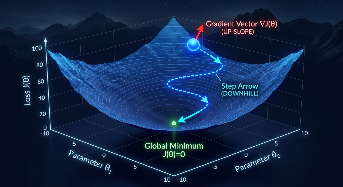
The gradient is the calculus hero of this story. It's the partial derivative of J(θ) with respect to every parameter in your model — a vector pointing in the direction of steepest increase. Here's the key insight: if you want to move downhill on the loss surface, you move in the opposite direction of the gradient. That minus sign in the update rule isn't arbitrary — it's the mathematical formalization of "go the other way."

The learning rate α is your step size, and it's simultaneously the most important and most underappreciated hyperparameter in deep learning. Too small: you make infinitesimal progress, training takes weeks, and you can get trapped in tiny local minima. Too large: you overshoot the valley entirely, bounce back and forth past the minimum, and loss oscillates wildly instead of decreasing. The "right" learning rate depends on your loss landscape's curvature, the batch size, the model architecture, and the training stage — which is why learning rate scheduling and adaptive optimizers like Adam exist.

📐 The Learning Rate Is Not One Number

Here's the thing most tutorials miss: in modern deep learning, the learning rate changes throughout training. Common strategies include: cosine annealing (smoothly decay from a high LR to near-zero), warm-up schedules (start tiny, ramp up, then decay — crucial for transformer training), and cyclical learning rates (oscillate between bounds, escaping local minima). The initial learning rate you set is really the maximum learning rate in a schedule, not a fixed value. Treating it as fixed is a beginner mistake that costs training efficiency and final model quality.

---

02The Update Rule: What Actually Happens on Every Training Step

The update rule θ = θ − α · ∇J(θ) looks deceptively simple. Let's trace exactly what happens at each training step. First, you take your current model weights (initialized randomly, or from a checkpoint). Second, you run a forward pass: feed your input data through the model, compute predictions, compare predictions to labels, and compute the loss scalar J. Third, you run a backward pass (backpropagation): compute the gradient of J with respect to every parameter, propagating derivatives backward through the computation graph via the chain rule. Fourth, you update every weight by subtracting α times its gradient. Repeat millions of times.

θ_new = θ_old − α · ∇J(θ_old)

One subtlety that trips people up: the gradient you compute is with respect to the current weights, not a global gradient. As the weights change, the loss landscape changes, and the gradient changes with it. You're not following a fixed path — you're following a path that reshapes itself with every step. This is why gradient descent doesn't guarantee finding the global minimum: the local gradient only tells you the direction of steepest descent from where you currently are.

Convergence happens when updates become negligibly small — mathematically, when ||∇J(θ)|| ≈ 0. Near a minimum, the loss surface is flat, the gradient is near zero, and updates shrink. In practice, you check for convergence by monitoring validation loss: if it stops improving for a set number of epochs (called patience in early stopping), you halt training. This prevents both under-training and over-training.

⚠️ Convergence ≠ Optimal Solution

Convergence means gradient ≈ 0. But gradient ≈ 0 can happen at three distinct places: a global minimum (best possible solution), a local minimum (good but not optimal), or a saddle point (gradient is zero but it's neither a min nor a max — extremely common in high-dimensional spaces). Modern neural network training frequently converges to saddle points, and often that's actually fine: research shows that many local minima in deep networks generalize similarly to the global minimum. Don't equate "converged" with "optimal."

gradient_descent.py

import numpy as np

def gradient_descent(X, y, lr=0.01, n_epochs=1000):
 """
 Batch gradient descent for linear regression.
 X: (n_samples, n_features), y: (n_samples,)
 """
 n, p = X.shape
 theta = np.zeros(p) # initialize weights at 0
 loss_history = []

 for epoch in range(n_epochs):
 # Forward pass: compute predictions and MSE loss
 y_hat = X @ theta # ŷ = Xθ
 errors = y_hat - y # residuals
 loss = (errors ** 2).mean() # MSE

 # Backward pass: compute gradient dJ/dθ
 gradient = (2 / n) * X.T @ errors # ∇J = (2/n) Xᵀε

 # Update rule: θ ← θ − α·∇J
 theta -= lr * gradient

 loss_history.append(loss)

 # Early convergence check
 if epoch > 10 and abs(loss_history[-2] - loss) < 1e-8:
 print(ff"Converged at epoch {epoch}")
 break

 return theta, loss_history

---

03Batch vs SGD vs Mini-Batch: Choosing Your Descent Style

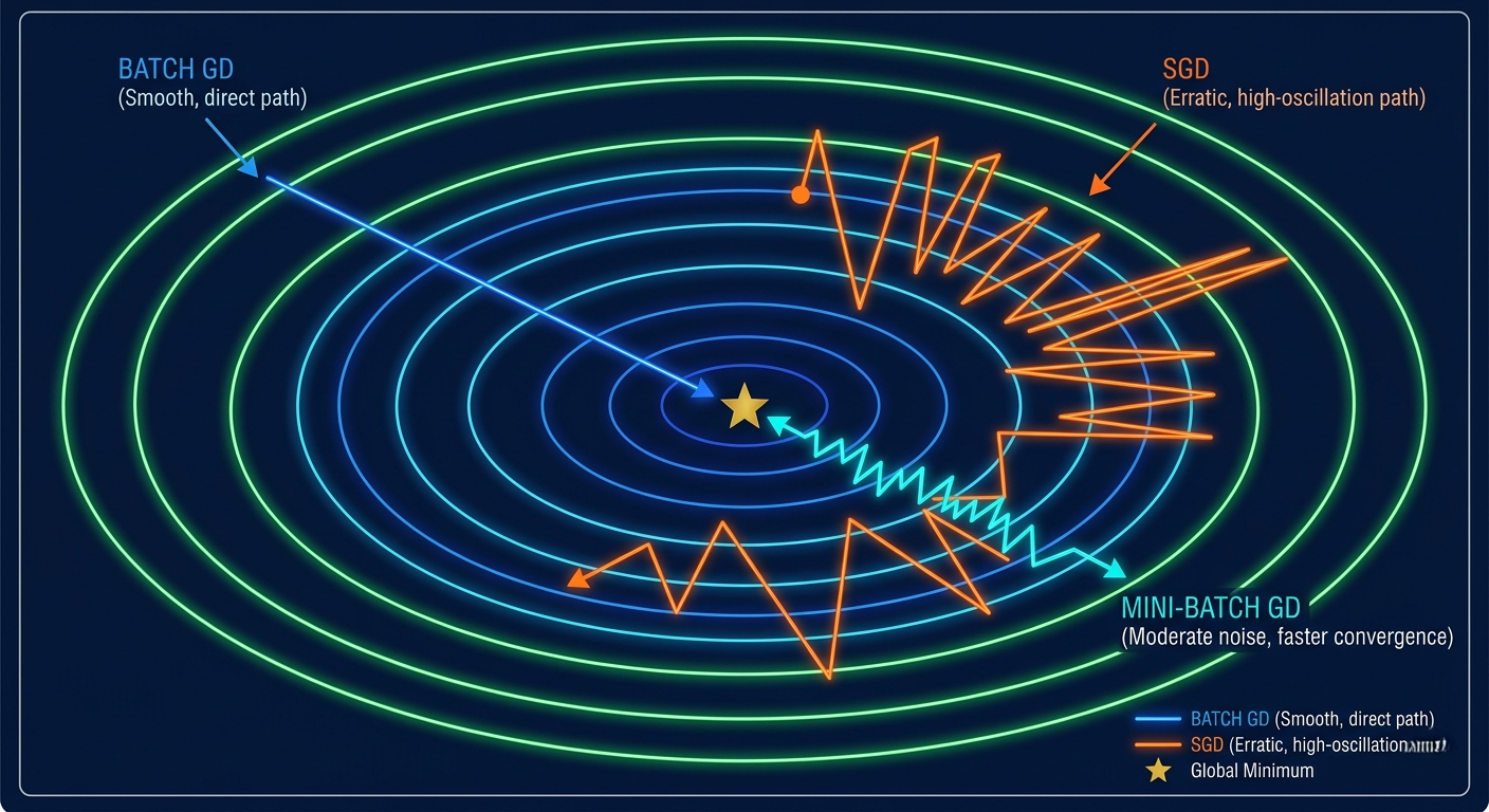
The gradient you compute for a weight update can be based on different amounts of data, and this choice has profound effects on training speed, memory use, and the quality of solutions found. The three variants are not just engineering tradeoffs — they have fundamentally different optimization dynamics.

Batch Gradient Descent computes the exact gradient over your entire dataset before updating weights. Imagine trying to navigate down a mountain using a perfect topographic map — every step is optimally chosen. The path is smooth and converges steadily. The problem: for datasets with millions of examples, computing the gradient over all of them before taking a single step is prohibitively expensive. One epoch (full pass through the data) might take hours. Also, if your loss surface has any local minima, you'll head straight into the nearest one.

Stochastic Gradient Descent (SGD) updates weights after every single training example. Imagine navigating with only a compass that shows a noisy, jittery reading — the direction is approximately right but bounces around. This noise is actually useful: it helps SGD escape shallow local minima and saddle points that batch GD would get trapped in. The downside is that the path is highly erratic, the loss zig-zags, and convergence is hard to detect cleanly. Mini-batch Gradient Descent — the real workhorse of modern deep learning — splits the dataset into small batches (typically 32, 64, or 128 examples), computes the gradient over each mini-batch, and updates. It averages out enough noise to be more stable than pure SGD, while being fast enough for large datasets and exploiting GPU vectorization.

💡 Why Batch Size Affects Generalization

Counterintuitively, smaller batch sizes often produce better-generalizing models than larger ones. Large batches (1024+) converge to sharp, narrow minima — the model memorizes specific patterns. Small batches converge to flat, wide minima — the model learns more generalizable features. The "sharpness" of a minimum correlates with how badly it overfits. This is why the conventional wisdom "use the largest batch that fits in GPU memory" is wrong for generalization: you want some noise in your gradient estimates. The sweet spot depends on your dataset and architecture, but 32-128 is usually a solid default.

---

04The Loss Landscape: Global Minima, Local Traps, and Saddle Points

In simple linear regression, the loss function (MSE) is convex — shaped like a perfect bowl with one global minimum. Life is easy. Gradient descent always converges to the optimal solution. But in neural networks with millions of parameters, the loss landscape is a high-dimensional terrain of breathtaking complexity: valleys, ridges, plateaus, and a menagerie of critical points where the gradient is zero but the solution quality varies enormously.

Local minima are points where the loss is lower than all neighboring points but not globally minimal. Early deep learning research worried extensively about local minima trapping gradient descent. More recent theoretical work has largely vindicated neural networks: in high dimensions, true local minima are rare. What you find more often is that all local minima of well-trained neural networks tend to have similar loss values, and the differences in generalization between them are small. The nightmare scenario of being trapped in a catastrophically bad local minimum rarely materializes in practice.

Saddle points are far more common and more problematic than local minima. A saddle point is a critical point (gradient = 0) where some directions curve upward and others curve downward — like a mountain pass. In two dimensions, saddle points are easy to escape. In a million-dimensional parameter space, saddle points can have hundreds of thousands of flat directions, creating vast "plateaus" where the gradient is nearly zero and learning is extremely slow. This is where the noise in SGD becomes valuable: it perturbs the trajectory just enough to escape these flat regions.

🔮 Myth: We Need to Find the Global Minimum

The goal of optimization in deep learning is not "find the global minimum." It's "find a minimum that generalizes well to new data." These are not the same thing. The global minimum of the training loss is usually an overfit solution — it has memorized the training set. The best generalizing solutions are typically in flat, wide minima that gradient descent with appropriate noise (mini-batch SGD) naturally finds. Chasing the absolute mathematical minimum is the wrong objective.

---

05Vanishing & Exploding Gradients: When Training Breaks Down

As gradients propagate backward through a deep network during backpropagation, they're multiplied at every layer by the layer's weight matrix and the derivative of its activation function. In deep networks with many layers, this repeated multiplication can cause catastrophic numerical behavior in two opposite directions.

Vanishing gradients occur when the products of these multiplications shrink toward zero. With sigmoid activations (which saturate at ±1 and have derivatives close to zero near saturation), gradients in early layers become so tiny that the weights there essentially stop updating. The first few layers of a 20-layer network with sigmoid activations learn nothing — they're frozen by vanishing gradients. This was a key barrier to training deep networks before 2010, and the primary reason ReLU activations (which have derivative exactly 1 for positive inputs) became dominant.

Exploding gradients are the opposite: repeated multiplication causes gradients to grow exponentially, eventually producing NaN (not a number) values that crash training. This is especially common in recurrent networks (RNNs) processing long sequences. The standard fix is gradient clipping: if the gradient norm exceeds a threshold, rescale it to that threshold. PyTorch and TensorFlow both provide this in one line. Modern architectures also use residual connections (ResNets), layer normalization, and careful weight initialization (Xavier/Kaiming) to prevent both pathologies.

⚠️ Signs Your Gradients Are Broken

Vanishing gradient symptoms: training loss stops decreasing after a few epochs despite not being near a minimum; early layers have near-zero gradient norms; loss curves are flat. Exploding gradient symptoms: training loss is NaN or Inf; loss jumps wildly between epochs; weights become very large very fast. Diagnostic tool: log the gradient norms for each layer during training. A healthy network should have gradient norms in a similar range across layers. Large discrepancies between early and late layers indicate gradient pathologies.

---

06Adaptive Optimizers: Momentum, RMSProp, and Adam

Vanilla gradient descent treats every parameter identically: same learning rate, same update magnitude. This is inefficient because different parameters in a neural network have vastly different gradient magnitudes and learning dynamics. Adaptive optimizers maintain per-parameter learning rates that automatically adjust based on gradient history.

Momentum adds a velocity term to gradient descent. Instead of jumping directly in the current gradient direction, you accumulate a weighted average of past gradients and use that for the update. Imagine rolling a ball down a hill: it builds up speed in consistent directions and dampens oscillations. Momentum is especially useful in narrow ravines — long, thin valleys common in deep learning loss landscapes — where vanilla GD would bounce back and forth across the narrow dimension rather than progressing along the valley floor.

RMSProp adapts per-parameter learning rates based on the root mean square of recent gradients. Parameters that have had consistently large gradients get a smaller effective learning rate; those with small gradients get a larger one. This addresses a key problem with vanilla SGD: sparse features (like rare words in NLP) receive tiny gradients and barely update, while frequent features receive large gradients and update too aggressively. Adam (Adaptive Moment Estimation) combines momentum with RMSProp: it maintains first-moment estimates (mean of past gradients, like momentum) and second-moment estimates (variance of past gradients, like RMSProp). With bias corrections for the early training warmup period, Adam is the most commonly used optimizer in production deep learning.

✅ Which Optimizer to Use in Practice

Default choice: Adam with lr=1e-3. It works reasonably well across architectures without tuning. For transformers (GPT, BERT, ViT): Adam with learning rate warmup is essentially required — the original Attention Is All You Need paper used it, and almost all subsequent work follows. For CNNs with careful tuning: SGD with momentum and cosine annealing often beats Adam on final performance (but requires more hyperparameter tuning). For RNNs: Adam or AdaGrad. The practical rule: start with Adam, use SGD+momentum for competitions and final production models where you want maximum performance and can afford tuning time.

optimizers_pytorch.py

import torch, torch.nn as nn

model = nn.Linear(10, 1)

# SGD with momentum
opt_sgd = torch.optim.SGD(model.parameters(),
 lr=0.01, momentum=0.9)

# RMSProp — good for RNNs
opt_rms = torch.optim.RMSprop(model.parameters(),
 lr=0.001, alpha=0.99)

# Adam — best default for most tasks
opt_adam = torch.optim.Adam(model.parameters(),
 lr=1e-3, betas=(0.9, 0.999))

# Training step (same for all optimizers):
for X, y in dataloader:
 opt_adam.zero_grad() # clear old gradients!
 loss = criterion(model(X), y)
 loss.backward() # backprop: compute ∇J
 torch.nn.utils.clip_grad_norm_( # clip if needed
 model.parameters(), max_norm=1.0)
 opt_adam.step() # θ = θ − α·∇J (with Adam magic)

---

07Feature Scaling: Why the Bowl Shape Is Everything

Imagine your loss function as a bowl, but someone squashed it badly — it's 1,000 meters deep but only 1 meter wide in one direction, and 1 kilometer wide in another. Gradient descent on this elongated bowl oscillates back and forth across the narrow dimension while making almost no progress along the wide dimension. That's exactly what happens when you run gradient descent on unscaled features.

When features have very different scales — say, house size in square feet (ranging 500–5000) and number of rooms (ranging 1–8) — the loss function's contours are elongated ellipses rather than circles. The gradient in the large-scale direction is huge; the gradient in the small-scale direction is tiny. The optimal learning rate for one is catastrophically wrong for the other. Gradient descent zigzags wildly in the large-scale direction while barely moving in the small-scale direction. Standardizing features (z = (x − μ) / σ) rounds out the bowl, makes all gradients comparable, and allows gradient descent to take direct paths to the minimum.

This is why standardization is mandatory before gradient-based optimization, but not strictly required for analytical OLS solutions (which solve the normal equations directly). The math of OLS doesn't care about feature scale — but gradient descent absolutely does. As a practical rule: if you're using any gradient-based optimizer (SGD, Adam, etc.), standardize your inputs. Period.

💡 Batch Normalization Is Feature Scaling at Every Layer

Batch Normalization (BatchNorm) can be thought of as applying feature scaling not just to inputs, but to the activations at every layer during training. It normalizes each layer's output to have zero mean and unit variance (within a mini-batch), then applies learnable scale and shift parameters. This dramatically stabilizes gradient flow: every layer in the network receives well-scaled inputs, preventing vanishing/exploding gradients and making very deep networks trainable. It's why training a 100-layer ResNet is feasible but training a 100-layer vanilla network without BatchNorm is essentially impossible.

---

synthesisHow It All Connects: The Complete Gradient Descent Picture

The gradient descent ecosystem is an interconnected web where every piece depends on the others. The loss function defines the landscape. The gradient tells you which way is "down." The learning rate controls how far you step. Mini-batch size determines how noisy (and thus exploratory) your descent is. Adaptive optimizers adjust per-parameter learning rates based on gradient history, solving the scale-sensitivity problem. Feature scaling makes the landscape bowl-shaped and explorable. Gradient clipping prevents pathological updates. And learning rate schedules adapt the step size as training progresses from coarse exploration to fine-grained convergence.

Understanding any one piece in isolation gives you a recipe to follow. Understanding how they interact gives you the judgment to diagnose failures, design training procedures, and push models beyond what the recipes allow. When your loss diverges, you know it's likely the learning rate. When early layers don't learn, you suspect vanishing gradients. When your model overfits despite high training loss, you consider larger batch sizes for smoother convergence. This is the difference between a practitioner and an engineer.

---

08Getting Started: Full Training Loop with PyTorch

full_training_loop.py

import torch, torch.nn as nn
from torch.utils.data import DataLoader, TensorDataset
import numpy as np

# ── 1. Data preparation with feature scaling ─────────────────
X_raw = np.random.randn(1000, 10)
X_raw[:, 0] *= 1000 # large scale feature
mu, sigma = X_raw.mean(axis=0), X_raw.std(axis=0)
X_scaled = (X_raw - mu) / sigma # standardize!

X = torch.FloatTensor(X_scaled)
y = torch.FloatTensor(np.random.randn(1000))
loader = DataLoader(TensorDataset(X, y), batch_size=64, shuffle=True)

# ── 2. Model ─────────────────────────────────────────────────
model = nn.Sequential(
 nn.Linear(10, 64), nn.ReLU(),
 nn.Linear(64, 32), nn.ReLU(),
 nn.Linear(32, 1)
)

# ── 3. Optimizer with learning rate schedule ─────────────────
optimizer = torch.optim.Adam(model.parameters(), lr=1e-3)
scheduler = torch.optim.lr_scheduler.CosineAnnealingLR(
 optimizer, T_max=50, eta_min=1e-6)
criterion = nn.MSELoss()

# ── 4. Training loop ─────────────────────────────────────────
for epoch in range(50):
 epoch_loss = []
 for X_b, y_b in loader:
 optimizer.zero_grad() # MUST clear grads
 loss = criterion(model(X_b).squeeze(), y_b)
 loss.backward() # compute ∇J
 torch.nn.utils.clip_grad_norm_( # prevent explosion
 model.parameters(), max_norm=1.0)
 optimizer.step() # θ -= α∇J
 epoch_loss.append(loss.item())
 scheduler.step() # decay lr
 if epoch % 10 == 0:
 print(ff"Epoch {epoch}: loss={np.mean(epoch_loss):.4f} lr={scheduler.get_last_lr()[0]:.6f}")

FAQFrequently Asked Questions

Why do we subtract the gradient instead of adding it? + The gradient points in the direction of steepest increase — toward higher loss values. Since we want to minimize the loss, we move in the opposite direction. The update rule θ = θ − α·∇J subtracts the gradient to move downhill. This is mathematically equivalent to following the negative gradient direction. If you accidentally added the gradient, your weights would update to maximize the loss — you'd be doing gradient ascent, which is the right approach when you want to maximize an objective (like reward in reinforcement learning) but wrong for supervised learning where you want to minimize prediction error. What happens to the gradient as you approach the minimum? + As you approach a minimum, the loss surface becomes flatter, and the gradient magnitude shrinks toward zero. Near the minimum, gradients approach zero from any direction since the surface is locally flat (approximately). This is both a blessing and a curse. It's a blessing because weight updates naturally become smaller as you converge, preventing oscillation around the minimum. It's a curse because if you're near a saddle point or plateau (which also have near-zero gradients), training slows dramatically even though you're far from a true minimum. This is why monitoring gradient norms alongside loss values is informative — a plateau in loss with near-zero gradients might mean you're at a minimum, or it might mean you're stuck at a saddle point. What is the difference between gradient descent and backpropagation? + Backpropagation and gradient descent are often confused but are fundamentally different things. Backpropagation is the algorithm that computes gradients — it uses the chain rule to efficiently propagate error derivatives backward through a neural network's computation graph, computing ∂J/∂θ for every parameter. Gradient descent is the optimization algorithm that uses those gradients to update parameters (θ = θ − α·∇J). Backprop answers "what are the gradients?" and gradient descent answers "how do we use those gradients to improve the model?" You could compute gradients via backprop but use them with any optimizer — Adam, RMSProp, etc. — that performs some version of gradient descent. Why is feature scaling important for gradient descent? + Without feature scaling, the loss function's contours are elongated ellipses where some directions have much steeper gradients than others. Gradient descent on an elongated loss surface zig-zags inefficiently: it makes large updates in high-gradient directions, overshooting, then correcting, while making tiny progress in low-gradient directions. The optimal step size for the steep direction is far too large for the shallow direction and vice versa. Standardizing features to zero mean and unit variance makes the loss contours roughly circular, allowing gradient descent to take more direct paths to the minimum and converge much faster. This is why the learning rate that "works" changes dramatically depending on whether your features are scaled. What is a saddle point and why does it matter? + A saddle point is a critical point (gradient ≈ 0) that's a minimum along some directions and a maximum along others — shaped like a horse saddle. In 2D, these are easy to escape with any perturbation. In the billion-parameter spaces of modern neural networks, saddle points can have hundreds of thousands of flat directions, creating vast plateaus where training appears to have converged but hasn't reached a minimum. Research suggests saddle points (not local minima) are the primary obstruction to gradient descent in deep learning. The noise in mini-batch SGD is crucial for escaping these plateaus. This is one reason why pure batch gradient descent — despite being mathematically cleaner — often performs worse than mini-batch SGD on deep networks. How do I know if my learning rate is too high or too low? + Too high: Training loss oscillates wildly or diverges (increases instead of decreasing). Loss might jump from reasonable values to NaN. Individual parameter values become very large. Too low: Loss decreases very slowly or appears to plateau early. Gradient norms are nonzero but loss barely moves. Training takes 10× longer than expected. The best diagnostic is to plot loss curves: a healthy training run shows monotonically decreasing loss (with some noise in mini-batch), stabilizing as it approaches a minimum. The learning rate range test (LR finder) is a standard technique: start with a tiny LR, increase it exponentially for one epoch, and plot loss vs LR. The sweet spot is typically just before the loss starts to diverge. Libraries like PyTorch Lightning include built-in LR finders. Is Adam always better than SGD? + Not always. Adam converges faster and requires less hyperparameter tuning, making it the better default for most users. But carefully tuned SGD with momentum often achieves better final generalization performance, particularly for image classification tasks. The reason: Adam's adaptive learning rates make it aggressive — it adapts quickly to gradient history and can find solutions that generalize less well. SGD with momentum is more conservative, tending to explore more of the loss landscape before settling. In competitive deep learning (Kaggle, academic papers), teams frequently start training with Adam for speed then switch to SGD for the final training phase to squeeze out better generalization. For transformers and NLP tasks, Adam (or AdamW, Adam with weight decay) is essentially always the choice. What is gradient clipping and when do I need it? + Gradient clipping caps the norm (magnitude) of the gradient vector at a maximum threshold before applying the update. If ||∇J|| > max_norm, rescale the gradient to ||∇J|| = max_norm while preserving its direction. This prevents exploding gradients from causing catastrophic weight updates and NaN losses. You should use gradient clipping: whenever training RNNs or LSTMs on sequences (exploding gradients are common), when training very deep networks (20+ layers), when fine-tuning pre-trained large models (their loss landscape can be steep), and generally as a defensive measure for any model that shows loss instability. PyTorch: torch.nn.utils.clip_grad_norm_(model.parameters(), max_norm=1.0). TensorFlow/Keras: set clipnorm=1.0 in your optimizer constructor.

🏔️ Optimization Lab

Four live experiments — tune hyperparameters, compare optimizers, and watch gradient descent descend in real time.

2D loss surface contour · colored ball = current position · click to teleport · trail shows path

Loss Landscape Explorer Learning Rate (α) 0.05 Landscape Type Gradient Noise (SGD) 0.00 — Current Loss 0 Steps — ||∇J|| Idle Status

Try: Set high LR and watch the ball overshoot and oscillate. Switch to Banana/Rosenbrock to see why momentum helps in elongated valleys. Add noise (SGD) on multimodal to escape local minima.

Loss curves for different learning rates — epoch vs loss

Learning Rate Impact LR 1 (too small) 0.001 LR 2 (good) 0.050 LR 3 (too large) 0.500 — LR1 final loss — LR2 final loss — LR3 final loss — Best LR

Loss vs epoch — optimizer comparison race

Trajectory on 2D loss surface

Optimizer Race Configuration Base Learning Rate 0.01 Noise (dataset) 0.30 Problem Type — SGD final loss — SGD+Momentum — Adam final loss — Winner

Training loss — with vs without gradient clipping under exploding gradient conditions

Gradient Clipping Simulator Gradient spike frequency 20% Spike magnitude 10× Clip threshold 1.0 — Without clipping — With clipping — NaN events — Gradient saves

Try: Set high spike frequency and magnitude. Without clipping, the training loss diverges to NaN (shown in red). With the threshold set correctly, clipping absorbs the spikes and training continues normally (shown in cyan).