Gradient Descent Explained: How Neural Networks Actually Learn

Gradient Descent & Learning · 3,600 words · 4 interactive labs · April 2026

Gradient Descent Explained:
How Neural Networks Actually Learn

You've heard "the network learns from data." But what does that mean, mathematically? Here's the honest, unvarnished story — cost functions, gradient descent, backpropagation, and the uncomfortable truth about what your network is really doing.

Read the Deep Dive ↓ Open Interactive Lab ⚗️ Table of Contents

1. Training Data & The Setup
2. Cost Functions: Measuring Failure
3. Gradient Descent: Rolling Downhill
4. Gradient Vectors: Relative Importance
5. 96% Accuracy — But Is It Smart?
6. The Uncomfortable Truth
7. Getting Started: Full Code
8. FAQ

// 01 Training Data & The Setup

Picture this: you've got a network with 13,000 weights and biases, all initialized to random values. You feed it a handwritten 3. The output layer lights up like a Christmas tree — not with the "3" neuron glowing bright, but with a chaotic mess of activations spread across all 10 output neurons. The network has no idea what it's doing. And right now, that's perfectly fine. That's the starting line.

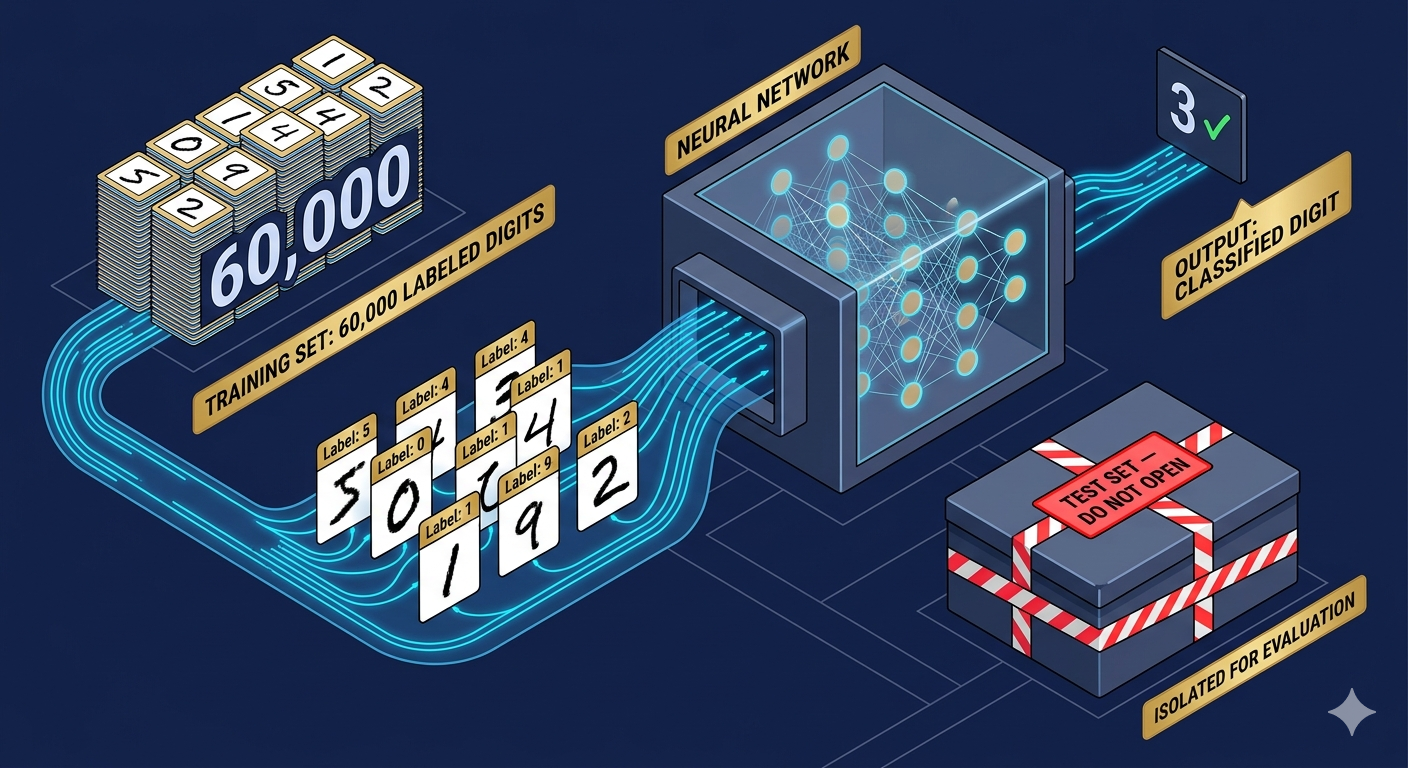
What makes neural networks remarkable isn't that they start smart — it's that they get smart through exposure to data. The MNIST dataset gives you 60,000 labeled training examples and 10,000 test examples: handwritten digits paired with the correct answer. The goal is to use these to systematically adjust all 13,000 parameters so the network gets progressively better at the task. The mechanism that does this adjusting is gradient descent, and understanding it changes how you think about machine learning at a fundamental level.

Here's an important distinction that most introductions gloss over: the training data and test data must be completely separate. You train on 60,000 examples, then you evaluate on 10,000 examples the network has never seen. The test accuracy is the only honest measure of whether the network actually learned something useful, or just memorized the training set. This split isn't a technicality — it's the entire integrity of the experiment.

💡 Pro Tip: The Train/Test Split Is Sacred

Never peek at your test set during development. Not to choose your architecture. Not to tune hyperparameters. Not even once. The moment you make any decision based on test performance, it becomes part of training and your evaluation is compromised. Use a validation set (a third split) for all development decisions.

data_setup.py

from torchvision import datasets, transforms
import torch

# Load MNIST — 60k train, 10k test
transform = transforms.Compose([
 transforms.ToTensor(),
 transforms.Normalize((0.1307,), (0.3081,)) # mean, std of MNIST
])

train_set = datasets.MNIST(root='.', train=True, download=True, transform=transform)
test_set = datasets.MNIST(root='.', train=False, download=True, transform=transform)

# Create a validation split from training data
n_val = 5000
train_set, val_set = torch.utils.data.random_split(
 train_set, [55000, n_val]
)

print(f"Train: {len(train_set):,} | Val: {len(val_set):,} | Test: {len(test_set):,}")
# → Train: 55,000 | Val: 5,000 | Test: 10,000

---

// 02 Cost Functions: Teaching a Computer to Feel Bad

Imagine you're coaching a new employee who's making decisions randomly. You can't just stare at them and hope they improve. You need a feedback signal — a specific, measurable way to tell them exactly how wrong they are. Cost functions are that feedback signal for neural networks.

Here's how it works: you feed the network a training image — say, a handwritten 3. The ideal output would be the "3" neuron at activation 1.0 and all other output neurons at 0.0. But with random weights, you get something like [0.2, 0.8, 0.3, 0.9, 0.1, 0.4, 0.3, 0.7, 0.2, 0.1] — complete nonsense. The cost function quantifies that nonsense. The simplest version is mean squared error (MSE): for each output neuron, compute (actual − desired)², then sum all 10 of those squared differences. The result is a single number that says "this is how badly you're doing right now."

The elegant insight is that this cost for a single example becomes a function of all 13,000 weights and biases. When you average it across all 60,000 training examples, you get a single scalar — the average cost — that compresses the network's entire performance into one number. The mission is now clear: find the combination of weights and biases that makes this number as small as possible. This is a pure optimization problem, and calculus has a lot to say about it.

⚠️ MSE vs Cross-Entropy: Which One To Use?

MSE works mathematically, but for classification tasks, cross-entropy loss is almost always better. Here's why: MSE treats all errors linearly, but cross-entropy penalizes confident wrong answers exponentially more than uncertain wrong answers — which matches how we intuitively want the network to learn. In PyTorch, use nn.CrossEntropyLoss() for multi-class classification.

• MSE: loss = Σ(output - target)² — simple but slow to train
• Cross-Entropy: loss = -Σ target · log(output) — faster convergence, gradient-friendly

cost_functions.py

import torch
import torch.nn as nn

# --- MSE Cost (original conceptual version) ---
def mse_cost(output, target_digit):
 # Create one-hot target: [0,0,0,1,0,0,0,0,0,0] for digit 3
 target = torch.zeros(10)
 target[target_digit] = 1.0
 return ((output - target) ** 2).sum()

# --- Cross-Entropy (production-grade, what you should use) ---
loss_fn = nn.CrossEntropyLoss()

# Example: network output for a batch of 64 images
outputs = torch.randn(64, 10) # logits from network
labels = torch.randint(0, 10, (64,)) # true digit labels
loss = loss_fn(outputs, labels)
print(f"Batch loss: {loss.item():.4f}") # ~2.3 at random init

---

// 03 Gradient Descent: Rolling Downhill in 13,000 Dimensions

Here's the thing most tutorials miss: gradient descent isn't specific to neural networks. It's a general algorithm for minimizing any function, and understanding it in the simplest possible case first makes the neural network version much less mysterious.

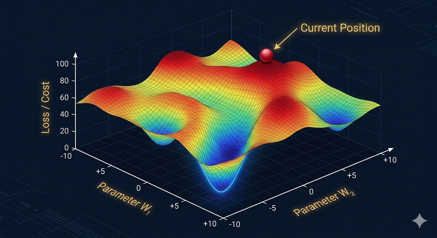
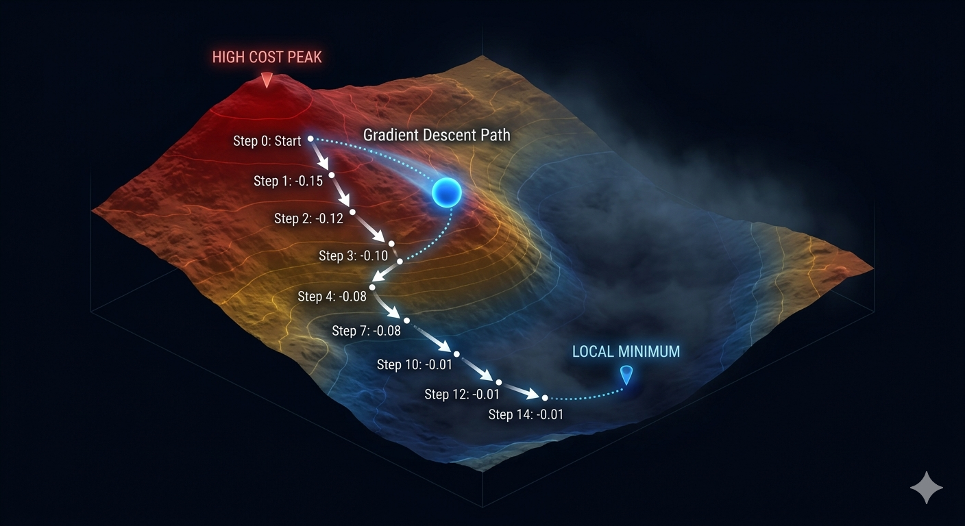
Imagine you're standing blindfolded on a hilly landscape. You want to reach the lowest point, but you can't see the terrain. What can you do? You can feel the slope under your feet. If the ground slopes upward to your left, you step right. If it slopes upward in front of you, you step backward. You always step in the direction that takes you downhill most steeply. That's gradient descent, literally. The gradient of a function at any point tells you the direction of steepest ascent. Negate it, and you get steepest descent. Take a small step in that direction. Repeat.

For a function of 13,000 variables — our neural network's weights and biases — the same principle applies, just in a space you can't visualize. The negative gradient is a 13,000-dimensional vector that tells you exactly how to nudge every single weight and bias to decrease the cost function most rapidly. The learning rate (usually a small number like 0.001) controls how big each step is. Too large and you overshoot the valley; too small and training takes forever. Choosing the right learning rate is part science, part art — and why things like Adam optimizer exist.

One crucial caveat: gradient descent finds a local minimum, not necessarily the global one. With 13,000 dimensions, there are potentially millions of valleys. Where you land depends on where you start (random initialization) and the path you take. Remarkably, for large neural networks this turns out to be mostly fine — research suggests most local minima in large networks are of roughly equal quality, and the real enemy is plateaus (flat regions where the gradient is nearly zero), not bad valleys.

✅ Learning Rate Intuition

Think of learning rate as your step size on the hillside. With a large step (e.g., 0.1), you might leap over the valley entirely and land on the other side — then back again — oscillating forever without converging. With a tiny step (e.g., 0.000001), you'll definitely reach the valley, but it'll take an eternity. The sweet spot (often around 1e-3 for Adam optimizer) gets you there quickly without overshooting.

gradient_descent.py

import torch
import torch.nn as nn

# The core gradient descent loop
model = nn.Sequential(nn.Flatten(), nn.Linear(784,16), nn.ReLU(),
 nn.Linear(16,16), nn.ReLU(), nn.Linear(16,10))
optimizer = torch.optim.SGD(model.parameters(), lr=0.01) # pure gradient descent
loss_fn = nn.CrossEntropyLoss()

for batch_X, batch_y in train_loader:
 # 1. Forward pass — compute predictions
 predictions = model(batch_X)

 # 2. Compute cost
 loss = loss_fn(predictions, batch_y)

 # 3. Backprop — compute gradient of cost w.r.t. all weights
 optimizer.zero_grad() # clear old gradients
 loss.backward() # the magic — computes ∂loss/∂w for every w

 # 4. Gradient descent step — nudge weights downhill
 optimizer.step() # w ← w - lr * ∂loss/∂w

---

// 04 What the Gradient Vector Is Really Telling You

The gradient isn't just a direction — it's a rich data structure encoding the relative importance of every parameter in your network. Consider a simplified example: a function with just two inputs, where the gradient at a particular point comes out as [3.0, 1.0]. That tells you two things simultaneously. First, you should nudge the first input in the negative direction (move downhill). Second, and more subtly: the first variable matters three times more than the second right now. A small change to it has three times the impact on the cost function.

Scale this up to 13,000 dimensions and the gradient vector becomes a priority list for your entire network. It's saying: "this weight matters a lot right now — adjust it significantly. This other weight barely matters — a tiny nudge is fine." This is why gradient descent is so much smarter than adjusting each weight randomly or by hand. It automatically focuses adjustment energy where it has the most impact.

This also explains why vanishing gradients are such a problem in deep networks. If the gradient component for a weight deep in the network is 0.00001 while a weight near the output has a gradient of 0.5, the early weight essentially stops learning. The gradient is telling you it doesn't matter — but it does, you're just not computing it accurately because of numerical issues compounding across many sigmoid activations. This is why ReLU exists, and why techniques like batch normalization and residual connections were invented.

🔥 Vanishing & Exploding Gradients

These are the two failure modes of gradient-based learning. Vanishing: gradients shrink exponentially as they propagate backward through many layers — early layers learn nothing. Exploding: gradients grow exponentially — weights fly off to infinity, training diverges. Solutions:

• Use ReLU or Leaky ReLU instead of sigmoid (helps vanishing)
• Gradient clipping: cap gradient norm at a threshold (fixes exploding)
• Careful weight initialization: Xavier/He init keeps scale stable
• Batch Normalization: normalizes layer outputs, stabilizes both problems

gradient_inspection.py

# After loss.backward(), inspect gradients
for name, param in model.named_parameters():
 if param.grad is not None:
 grad_norm = param.grad.norm().item()
 print(f"{name:30s} | grad_norm: {grad_norm:.6f}")

# Output might look like:
# 0.weight | grad_norm: 0.000034 ← vanishing!
# 0.bias | grad_norm: 0.000021
# 2.weight | grad_norm: 0.002143
# 4.weight | grad_norm: 0.089234 ← healthy

# Fix exploding gradients with clipping
torch.nn.utils.clip_grad_norm_(model.parameters(), max_norm=1.0)

---

// 05 96% Accuracy — But Is This Network Actually Smart?

After training our simple two-hidden-layer network (784 → 16 → 16 → 10) on MNIST, you'll typically see around 96% test accuracy. Bump the hidden layer sizes, tweak the learning rate, train a bit longer, and you can push it to 98%. That sounds impressive. But here's the counterintuitive part: this accuracy masks a deeply shallow kind of "intelligence."

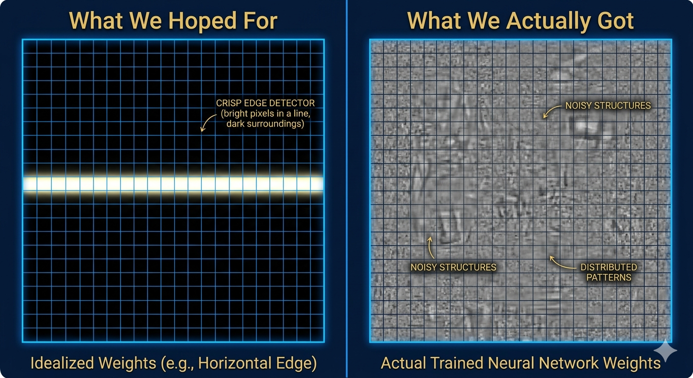
When researchers visualize what the hidden layer neurons are responding to — by examining the weights connecting each hidden neuron to the input pixels — what they find is... mostly noise. The weights don't show clean edge detectors. They don't show clearly interpretable patterns. They show vaguely patterned blobs that somehow, collectively, combine to correctly classify digits most of the time. The network found a local minimum that works, but it's not the elegant, interpretable solution we hoped for.

The damning test: feed the trained network a completely random noise image. A truly intelligent digit recognizer should respond with something like "I don't know — this doesn't look like any digit." Instead, our network confidently identifies the noise as a specific digit, often with high certainty. It's not recognizing digits — it's recognizing mathematical patterns in the weight-space that happen to correlate with digits in the training distribution. Step outside that distribution and the facade crumbles immediately.

⚠️ The Memorization Bombshell

A 2017 paper by Zhang et al. demonstrated something disturbing: a neural network trained on MNIST with randomly shuffled labels can still achieve near-perfect training accuracy. The network just memorizes the random mapping. It achieves zero test accuracy (obviously), but training accuracy is perfect. This proves that minimizing the training loss doesn't guarantee learning anything meaningful — the network is powerful enough to memorize noise. This is why generalization and test performance are everything.

evaluate.py

# Test the "random noise" failure case
model.eval()
with torch.no_grad():

 # Feed completely random noise
 noise = torch.rand(1, 1, 28, 28)
 output = torch.softmax(model(noise), dim=1)
 pred, conf = output.max(1)
 print(f"Noise classified as: {pred.item()} ({conf.item()*100:.1f}% confident)")
 # → "Noise classified as: 5 (74.3% confident)" ← deeply wrong

 # Proper test set evaluation
 correct = sum(model(x).argmax(1) == y
 for x, y in test_loader)
 print(f"Test accuracy: {correct/len(test_set)*100:.2f}%")
 # → "Test accuracy: 96.12%"

---

// 06 The Uncomfortable Truth About What's Really Happening

Let's synthesize the uncomfortable truth that emerges from studying gradient descent carefully. The network isn't "learning" in the rich cognitive sense. It's finding parameters that minimize a mathematical function on a specific dataset. The fact that this also makes it useful in the real world is a happy consequence of the dataset reflecting real-world structure — not evidence of genuine understanding.

Interestingly, research shows that structured data makes gradient descent easier. When you train a network on properly labeled MNIST, the training loss drops fast — you find a good minimum quickly. When you train on randomly labeled MNIST, the loss drops painfully slowly (near-linear decline), even though the network eventually "memorizes" the random mapping. This suggests gradient descent is doing something smarter than pure memorization: it's exploiting the structure of the data to find shortcuts to good solutions. Good news, but don't mistake efficiency for intelligence.

This is why convolutional neural networks (CNNs) so dramatically outperform plain fully-connected networks on image tasks: they build in structural assumptions about images (local patterns matter, position-invariance matters) that match reality. The network's architecture itself becomes a form of prior knowledge. The plain network has to discover these inductive biases from scratch, and with enough capacity, it can — but inefficiently, and without the clean interpretability we'd want.

✅ The Path Forward

Understanding these limitations is why the field moved from plain networks to CNNs (for images), RNNs and Transformers (for sequences), and Graph Neural Networks (for relational data). Each architecture embeds domain-specific inductive biases that make learning faster, more data-efficient, and more interpretable. The plain network described here is the necessary foundation — not the destination.

---

// 07 Getting Started: Complete Working Example

Here's a production-quality script that implements everything discussed — with training, validation, gradient inspection, and the noise test. Run it yourself and watch gradient descent work in real time.

full_training.py

import torch, torch.nn as nn
from torchvision import datasets, transforms
from torch.utils.data import DataLoader, random_split

# ── Data ─────────────────────────────────────
T = transforms.Compose([transforms.ToTensor(),
 transforms.Normalize((0.1307,),(0.3081,))])
full = datasets.MNIST('.', train=True, download=True, transform=T)
test = datasets.MNIST('.', train=False, download=True, transform=T)
train, val = random_split(full, [55000, 5000])
tr_loader = DataLoader(train, batch_size=64, shuffle=True)
va_loader = DataLoader(val, batch_size=256)
te_loader = DataLoader(test, batch_size=256)

# ── Model ─────────────────────────────────────
model = nn.Sequential(
 nn.Flatten(),
 nn.Linear(784, 64), nn.ReLU(), nn.Dropout(0.2),
 nn.Linear(64, 32), nn.ReLU(), nn.Dropout(0.2),
 nn.Linear(32, 10),
)

# ── Training ──────────────────────────────────
opt = torch.optim.Adam(model.parameters(), lr=1e-3)
loss_fn = nn.CrossEntropyLoss()

for epoch in range(10):
 model.train()
 train_loss = 0
 for X, y in tr_loader:
 loss = loss_fn(model(X), y)
 opt.zero_grad(); loss.backward(); opt.step()
 train_loss += loss.item()

 model.eval()
 with torch.no_grad():
 val_acc = sum(model(x).argmax(1).eq(y).sum().item()
 for x,y in va_loader) / 5000
 print(f"Epoch {epoch+1:2d} | loss {train_loss/len(tr_loader):.4f} | val {val_acc*100:.2f}%")

On a modern laptop CPU, this trains in under 2 minutes and reaches ~98% validation accuracy. The interactive lab below lets you see gradient descent happen visually, in real time, without writing a single line of code.

// synthesisHow It All Connects

The full picture: a neural network is a function of 13,000 parameters (weights and biases). A cost function wraps that to produce a single scalar measuring how bad the current parameters are. Gradient descent reads the cost function's gradient — a 13,000-dimensional vector — to find the direction of fastest decrease. Backpropagation efficiently computes that gradient using the chain rule. Training is repeating this loop thousands of times across all training examples. The result is a set of weights that minimize the cost on training data and, hopefully, generalizes to new data.

The caveats are real: the network may not learn what we hoped it would. It may memorize. It may be fooled by noise. It may find a local minimum that works but isn't interpretable. These aren't bugs to fix — they're the nature of gradient-based optimization on finite data. Understanding them is what separates a machine learning practitioner from someone who just runs training scripts and hopes for the best.

---

// FAQFrequently Asked Questions

What's the difference between gradient descent and backpropagation? + They're often conflated but they're different things. Gradient descent is the optimization algorithm: take a step in the direction of the negative gradient, repeat. Backpropagation is the efficient algorithm for computing that gradient — it uses the chain rule of calculus to propagate error signals backward through the network. You need backpropagation to compute the gradient; you use gradient descent to act on it. What is stochastic gradient descent (SGD) and why use it instead of full gradient descent? + Full gradient descent computes the gradient by averaging across all training examples before taking one step. For 60,000 examples, that's expensive and slow. Stochastic gradient descent (SGD) estimates the gradient using just a single random example. Mini-batch SGD (the standard practice) uses a small batch of 32–256 examples, balancing speed and accuracy of the gradient estimate. The stochasticity (randomness) from mini-batches actually helps — it prevents getting stuck in sharp, narrow minima and often finds flatter minima that generalize better. Why does the learning rate matter so much? + The learning rate directly controls the size of each parameter update. Too high: updates overshoot minima, loss oscillates or diverges. Too low: convergence takes impractically long and you may get trapped in plateaus. In practice, use learning rate schedules (start high, decay over time) or adaptive optimizers like Adam, which adjusts the effective learning rate per-parameter automatically based on historical gradient magnitudes. Most practitioners start with Adam at lr=1e-3 and tune from there. Can gradient descent get trapped in bad local minima? + Theoretically yes, practically — for large networks — usually no. Research by Choromanska et al. (2015) suggests that in high-dimensional loss landscapes (lots of parameters), most local minima are "good" (close to global minimum quality). The bigger practical enemies are saddle points (not local minima, but zero-gradient flat spots) and plateaus. SGD's stochasticity helps escape both. For small networks like our 784→16→16→10 example, bad local minima are more of a real concern. What is overfitting and how do I know if it's happening? + Overfitting is when the network memorizes the training data instead of learning generalizable patterns. The telltale sign: training loss keeps decreasing while validation loss starts increasing. The gap between them is the overfit signal. Solutions in order of preference: more training data, data augmentation, dropout regularization, L2 weight decay, reducing model capacity, or early stopping (stop training when validation loss stops improving). What is Adam optimizer and why is it better than plain SGD? + Adam (Adaptive Moment Estimation) combines two ideas: momentum (accumulates velocity in the gradient direction, like a ball that doesn't stop immediately) and RMSProp (adapts learning rate per-parameter based on recent gradient magnitudes). The result is an optimizer that's much less sensitive to learning rate choice, converges faster, and handles sparse gradients well. It's not always better than SGD+momentum (some tasks, especially vision, see better final performance with tuned SGD), but it's more forgiving — a great default. Why does the network confidently classify random noise? + Because the cost function gave it zero incentive to be uncertain. During training, every single input was a real digit with a correct label — the network never saw "none of the above." Its output space is constrained to 10 options, so even random input activations produce a distribution over those 10 options. The softmax function normalizes these to sum to 1.0, so something always has high probability. True uncertainty (outputting near-uniform distribution for out-of-distribution inputs) requires explicit training for it, which techniques like confidence calibration and out-of-distribution detection address. How does backpropagation actually work? + Backpropagation uses the chain rule of calculus to compute how the cost function changes with respect to each weight and bias. Starting from the output (where you know the error), it propagates "credit" backward through each layer: how much did this layer's weights contribute to the final error? Because neural networks are composed functions (layer after layer), the chain rule naturally decomposes into layer-by-layer gradient computation. The math is elegant but dense — it's the subject of a dedicated deep-dive post in this series.

⚗️ Interactive Lab

Four experiments to build real intuition about gradient descent, cost functions, and how your choices affect learning — no code required.

Click anywhere on the surface to place the starting point, then hit Run.

Gradient Descent Controls Learning Rate 0.050 Momentum 0.00 Max Steps 80 Surface Type 0 Steps — Loss — x position — y position Try this: Set LR very high (>0.15) and watch it overshoot. Add momentum and watch convergence speed up. Switch to "Saddle Point" to see where descent gets confused.

Cost surface over 2 weight dimensions — all others held fixed

Training loss curve over gradient descent steps

Training Simulation Learning Rate 0.010 Batch Size 32 Noise (SGD variance) 0.15 0 Epoch 2.302 Avg Loss 10% Est. Accuracy Idle Status Draw a Digit Output Confidences Network State ? Prediction — Confidence 12,960 Parameters 4 Layers Hidden Size 16 Activation Try: Draw a clear "3", classify it. Then click "Add Noise" and classify again — watch confidence change. Then clear and draw random scribbles to see the network's overconfident misclassification. Neuron Weight Map — Layer 1→2

Green = positive weight · Red = negative weight · Hover to inspect

Activation Function Shapes

Compare how different activation functions transform the weighted sum

Select Neuron to Inspect Neuron Index 0 Weight Scale (init) 1.0× — Pos Weights — Neg Weights — Max Weight — Min Weight