
In 2012, Netflix's recommendation engine was producing blatantly wrong suggestions for millions of users. The problem wasn't the ML model — it was the data feeding it. Batch jobs were failing silently, historical watch data was going stale, and real-time viewing events weren't being incorporated into recommendations fast enough. A user could watch three episodes of a show and still be recommended that same show as if they'd never seen it. The recommendation engine was only as good as the data pipeline supplying it — and that pipeline was broken in ways nobody had built monitoring to detect.
Most organizations have some version of this problem. They have data — enormous amounts of it — sitting in databases, streaming from applications, arriving from IoT sensors, accumulating in log files. They have analytics teams who want to query it, ML teams who want to train on it, executives who want dashboards from it. And in between the raw data and the people who need it, there's a mess of scripts, scheduled jobs, ad-hoc ETL processes, and fragile dependencies that someone called a "data pipeline" — mostly because that sounds better than "a collection of cronjobs that we're all afraid to touch."
A real data pipeline is an engineered system — designed, monitored, and maintainable — that takes raw, messy data from wherever it lives and transforms it into clean, structured, accessible information that drives decisions. This post covers the complete architecture: the five stages every data pipeline goes through (collect, ingest, store, compute, consume), the technologies that power each stage, the design decisions that separate robust pipelines from brittle ones, and the practical code to get started.
Table of Contents
- Data Collection: The Sources That Feed Everything
- Data Ingestion: Loading Data Into the Pipeline Environment
- Batch Processing vs Stream Processing: Choosing the Right Compute Model
- ETL and ELT: Transforming Messy Data Into Reliable Structure
- Data Storage: Lakes, Warehouses, and Lakehouses
- Data Consumption: Turning Data Into Decisions
- How It All Connects: The Complete Data Pipeline Architecture
- Getting Started: Building Your First Data Pipeline
- FAQ
- Conclusion
Data Collection: The Sources That Feed Everything
Every data pipeline starts with a fundamental question: where is your data, and what form does it take? The answer determines every downstream architectural decision. Data doesn't arrive from one place in one format at one rate — it arrives from dozens of sources, in incompatible formats, at wildly different velocities, with different reliability characteristics. Building a pipeline that handles this heterogeneity without creating a maintenance nightmare is the first engineering challenge.
Transactional data stores — MySQL, PostgreSQL, DynamoDB, Oracle — are where your application's ground truth lives. Every user registration, every order placed, every payment processed, every inventory update: it all lands in a transactional database first. These databases are optimized for reads and writes at the row level (OLTP — Online Transaction Processing), not for the analytical queries (OLAP) that your data team wants to run. Joining five tables across 50 million rows to compute monthly revenue by geographic region while your production database is also handling live checkout requests is a recipe for taking down your application. This is why data has to move: analytical workloads need a different storage layer than operational workloads.
Data streams capture events as they happen — not a snapshot of a database table, but a continuous flow of things occurring in your system. User clicks, search queries, page views, API calls, clickstream events, sensor readings, log entries — these are generated continuously, at high volume, and their value is often time-sensitive. A fraud detection system that analyzes a suspicious transaction 10 minutes after it happened is useful. One that analyzes it 2 milliseconds after it happened can actually stop it. Apache Kafka and Amazon Kinesis are the dominant technologies for capturing and buffering these event streams, providing durable, scalable message queues that decouple the systems generating events from the systems consuming them.
Application-generated data — logs, metrics, API responses, third-party data from marketing platforms, CRM systems, payment processors — rounds out the picture. This data often comes in inconsistent formats (JSON, XML, CSV, binary protocols), on unpredictable schedules, with quality varying from pristine to genuinely chaotic. A SaaS company might collect data from its own application, from Stripe's webhook events, from Salesforce's API, from Google Analytics exports, and from customer-uploaded CSV files — all in the same pipeline. The collection layer has to handle this diversity without losing data or propagating bad data downstream.
# Illustrating three collection patterns for an e-commerce data pipeline

import boto3
import mysql.connector
from kafka import KafkaProducer
import json
from datetime import datetime

# ============================================================
# Pattern 1: Pull from transactional database (batch collection)
# ============================================================
def collect_from_mysql(last_extracted_at: str) -> list[dict]:
    """
    Incremental extraction from operational database.
    Always use WHERE clause — never SELECT * from a 50M row table.
    """
    conn = mysql.connector.connect(
        host='prod-db.internal', database='ecommerce',
        user='readonly_user', password='...'  # read-only credentials!
    )
    cursor = conn.cursor(dictionary=True)

    # Incremental extraction: only fetch records since last run
    # Critical: use indexed column (updated_at) to avoid full table scans
    query = """
        SELECT order_id, user_id, total_amount, status,
               created_at, updated_at, shipping_address
        FROM orders
        WHERE updated_at > %s
        ORDER BY updated_at ASC
        LIMIT 10000
    """
    cursor.execute(query, (last_extracted_at,))
    orders = cursor.fetchall()

    conn.close()
    print(f"Collected {len(orders)} orders updated since {last_extracted_at}")
    return orders

# ============================================================
# Pattern 2: Real-time event stream collection via Kafka
# ============================================================
producer = KafkaProducer(
    bootstrap_servers=['kafka:9092'],
    value_serializer=lambda v: json.dumps(v).encode('utf-8'),
    acks='all'  # durability guarantee
)

def collect_user_event(event_type: str, user_id: str, data: dict):
    """
    Collect real-time user events into Kafka stream.
    Called directly from application code on every user action.
    """
    event = {
        'event_id': f"{user_id}-{datetime.utcnow().timestamp()}",
        'event_type': event_type,
        'user_id': user_id,
        'timestamp': datetime.utcnow().isoformat(),
        'data': data,
        'source': 'web-app-v2'
    }
    producer.send(f'user-events.{event_type}', value=event)
    # Non-blocking: application doesn't wait for Kafka confirmation

# Called on every user action in the application:
collect_user_event('product_viewed', 'user-123', {
    'product_id': 'PROD-456', 'category': 'electronics',
    'price': 299.99, 'page_position': 3
})
collect_user_event('search', 'user-123', {
    'query': 'wireless headphones', 'results_count': 48
})

# ============================================================
# Pattern 3: Pull from third-party API (application data)
# ============================================================
def collect_from_stripe_webhooks(webhook_payload: dict) -> dict:
    """
    Collect payment events from Stripe webhooks.
    Webhooks push to your endpoint; you collect and normalize.
    """
    event_type = webhook_payload['type']
    data = webhook_payload['data']['object']

    # Normalize Stripe's format to your internal schema
    normalized = {
        'payment_id': data.get('id'),
        'amount_cents': data.get('amount'),
        'currency': data.get('currency'),
        'status': data.get('status'),
        'customer_id': data.get('customer'),
        'created_at': datetime.fromtimestamp(data.get('created')).isoformat(),
        'source': 'stripe',
        'raw_event': event_type
    }
    return normalized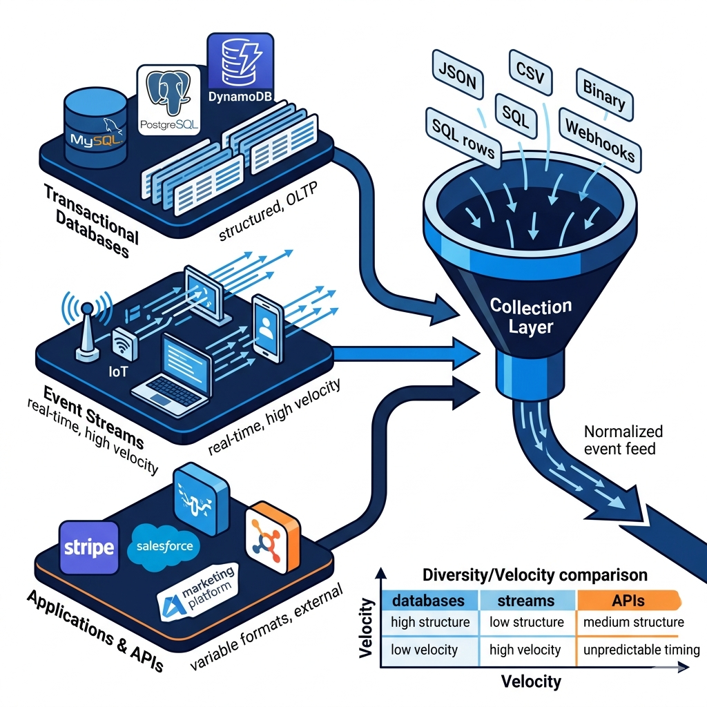
Pro Tips & Common Mistakes — Data Collection
Pro Tip: Always use incremental extraction from operational databases — never full dumps. A full SELECT on a 100M-row table at 2 a.m. will lock tables, spike database load, and take hours. Incremental extraction using an indexed
updated_atorcreated_atcolumn collects only what changed since the last run. Track your last extraction timestamp in a state store (a simple table, S3 file, or pipeline metadata store) and use it as your WHERE clause lower bound. For complex change detection, look into CDC (Change Data Capture) tools like Debezium, which capture database changes via the transaction log rather than query polling.
Common Mistake: Collecting data using full admin credentials instead of read-only service accounts. Your data collection processes shouldn't have write access to production databases. Create dedicated read-only database users, scope API credentials to the minimum necessary permissions, and treat data collection credentials as the security-sensitive secrets they are. A compromised collection job with admin credentials can corrupt production data. One with read-only credentials can't.
Data Ingestion: Loading Data Into the Pipeline Environment
Collecting data and ingesting it are different operations that tutorials often conflate. Collection is acquiring data from its source. Ingestion is loading that data into your pipeline's processing environment — which might mean different things depending on whether you're handling batch data or streaming data, and what your downstream compute layer expects.
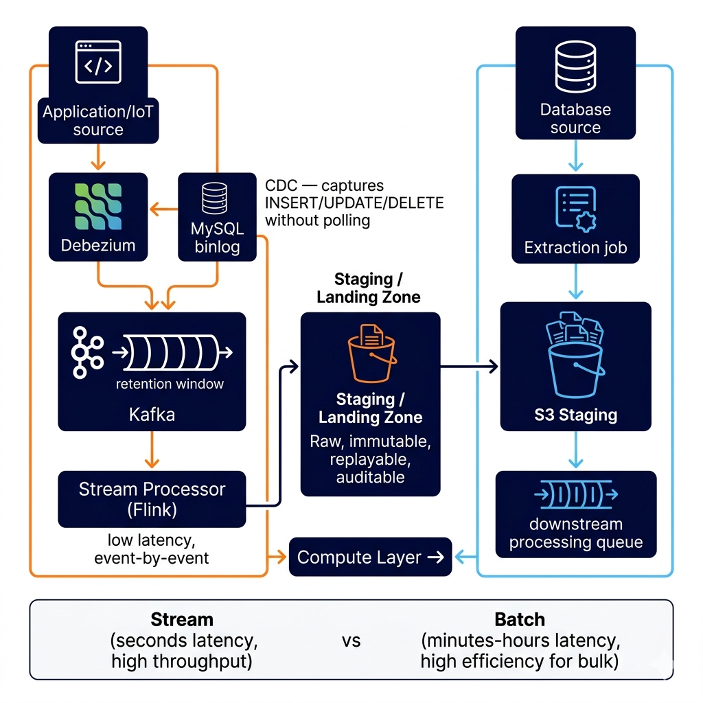
For real-time streaming data, ingestion typically means routing events through a message queue infrastructure before they reach any processing system. Apache Kafka and Amazon Kinesis serve as durable buffers that decouple the systems generating events (your web application, IoT devices, mobile apps) from the systems consuming them (Flink stream processors, Lambda functions, real-time ML models). This decoupling is critical: if your stream processor is down for 10 minutes for a deployment, events don't disappear — they accumulate in Kafka, and when the processor comes back up, it picks up exactly where it left off. The ingestion layer acts as the shock absorber for the entire pipeline.
For batch data from databases, ingestion often involves Change Data Capture (CDC) — a technique that captures row-level changes (inserts, updates, deletes) from the database's transaction log rather than querying the database directly. Debezium, a popular open-source CDC tool, connects to MySQL's binary log, PostgreSQL's write-ahead log, or MongoDB's oplog and publishes every change event to Kafka in real time. This approach has several advantages over query-based extraction: it captures deletes (which a WHERE updated_at > X query misses), introduces almost zero load on the source database, and provides truly real-time change propagation rather than periodic batch refreshes. Many modern data platforms are moving to CDC-first ingestion precisely because it eliminates the entire category of "how do we know what changed?" problems.
The ingestion phase is also where you make a critical architectural decision: does data go directly to processing, or does it land in intermediate storage first? For real-time streaming workloads, data typically flows directly from Kafka to stream processors without touching storage. For batch workloads, data is often written to a staging area (an S3 bucket, HDFS, or a landing zone in your data lake) before processing begins. This staging pattern provides durability (if processing fails, raw data is still there to replay), auditability (you have a record of exactly what raw data looked like before any transformations), and flexibility (multiple downstream processes can read from the same staging area independently).
# Data ingestion patterns — CDC with Debezium and batch staging

# ============================================================
# Pattern 1: CDC-based ingestion via Debezium (reads MySQL binlog)
# Debezium publishes changes to Kafka; we consume and land in staging
# ============================================================
from kafka import KafkaConsumer
import json
import boto3
from datetime import datetime

# Debezium automatically creates topics like: dbserver1.ecommerce.orders
CDC_TOPIC = 'dbserver1.ecommerce.orders'

def ingest_cdc_events_to_staging():
    """
    Consume CDC events from Debezium and write to S3 staging.
    Debezium captures INSERT/UPDATE/DELETE without polling the DB.
    """
    consumer = KafkaConsumer(
        CDC_TOPIC,
        bootstrap_servers=['kafka:9092'],
        group_id='cdc-ingestion-pipeline',
        auto_offset_reset='earliest',
        value_deserializer=lambda m: json.loads(m.decode('utf-8'))
    )

    s3 = boto3.client('s3')
    batch = []
    BATCH_SIZE = 1000

    for msg in consumer:
        event = msg.value

        # Debezium event structure: op = 'c'(reate), 'u'(pdate), 'd'(elete), 'r'(ead)
        operation = event.get('op')
        before = event.get('before')  # state before change (UPDATE/DELETE)
        after = event.get('after')    # state after change (INSERT/UPDATE)

        # Normalize to pipeline's internal event format
        ingestion_record = {
            'ingested_at': datetime.utcnow().isoformat(),
            'source_table': 'orders',
            'operation': operation,
            'before': before,
            'after': after,
            'source_ts_ms': event.get('ts_ms'),
            'transaction_id': event.get('transaction', {}).get('id')
        }

        batch.append(ingestion_record)

        if len(batch) >= BATCH_SIZE:
            # Write batch to S3 staging (raw landing zone)
            s3_key = f"staging/cdc/orders/{datetime.utcnow().strftime('%Y/%m/%d/%H')}/{msg.offset}.json"
            s3.put_object(
                Bucket='data-lake-raw',
                Key=s3_key,
                Body='\n'.join(json.dumps(r) for r in batch).encode()
            )
            print(f"Landed {len(batch)} CDC events to s3://{s3_key}")
            batch = []


# ============================================================
# Pattern 2: Batch ingestion with staging and validation
# ============================================================
import pandas as pd
from dataclasses import dataclass
from typing import List

@dataclass
class IngestionResult:
    records_ingested: int
    records_rejected: int
    staging_location: str
    errors: List[str]

def ingest_batch_to_staging(source_records: list[dict],
                            dataset_name: str,
                            run_id: str) -> IngestionResult:
    """
    Batch ingestion with validation and staging.
    Raw data lands in S3 before any transformation — enables replay.
    """
    errors = []
    valid_records = []

    for record in source_records:
        # Basic ingestion-time validation (not deep transformation)
        if not record.get('order_id'):
            errors.append(f"Missing order_id: {record}")
            continue
        if not isinstance(record.get('total_amount'), (int, float)):
            errors.append(f"Invalid amount for order {record.get('order_id')}")
            continue

        # Add pipeline metadata
        record['_ingested_at'] = datetime.utcnow().isoformat()
        record['_pipeline_run_id'] = run_id
        record['_source'] = 'mysql.orders'
        valid_records.append(record)

    # Write to staging in Parquet format (efficient for large-scale storage)
    df = pd.DataFrame(valid_records)
    staging_path = f"s3://data-lake-raw/{dataset_name}/{run_id}/data.parquet"

    # Write Parquet to S3 (in practice, use boto3 + PyArrow or Spark)
    df.to_parquet('/tmp/staging.parquet', engine='pyarrow', index=False)
    # boto3 upload would follow here

    return IngestionResult(
        records_ingested=len(valid_records),
        records_rejected=len(errors),
        staging_location=staging_path,
        errors=errors[:10]  # cap error log size
    )
Pro Tips & Common Mistakes — Data Ingestion
Pro Tip: Write raw data to a staging/landing zone in your data lake before any transformation, even for batch pipelines. This raw layer — immutable, partitioned by ingestion date, stored in Parquet or JSONL — is your insurance policy. When (not if) a transformation bug corrupts downstream data, you can replay from the raw layer without re-extracting from source systems that may have changed or been overwritten. Many teams only realize they need this insurance after their first production data corruption incident.
Common Mistake: Not implementing CDC and instead relying on
updated_attimestamp-based polling to detect changes. This approach silently misses hard deletes (rows removed from the database), requires source tables to have anupdated_atcolumn (not all do), and introduces poll-interval latency (anything from 1 minute to 1 hour of delay). CDC reads the database's transaction log directly — it catches all changes including deletes, introduces near-zero database load, and propagates changes in real time. Tools like Debezium make CDC implementation straightforward for MySQL, PostgreSQL, and MongoDB.
Batch Processing vs Stream Processing: Choosing the Right Compute Model
With data ingested, it needs to be processed — and the single most important architectural decision in a data pipeline is whether to use batch processing or stream processing (or both, in a Lambda or Kappa architecture). These aren't just different technologies; they represent fundamentally different computational models with different latency profiles, consistency guarantees, and operational characteristics.
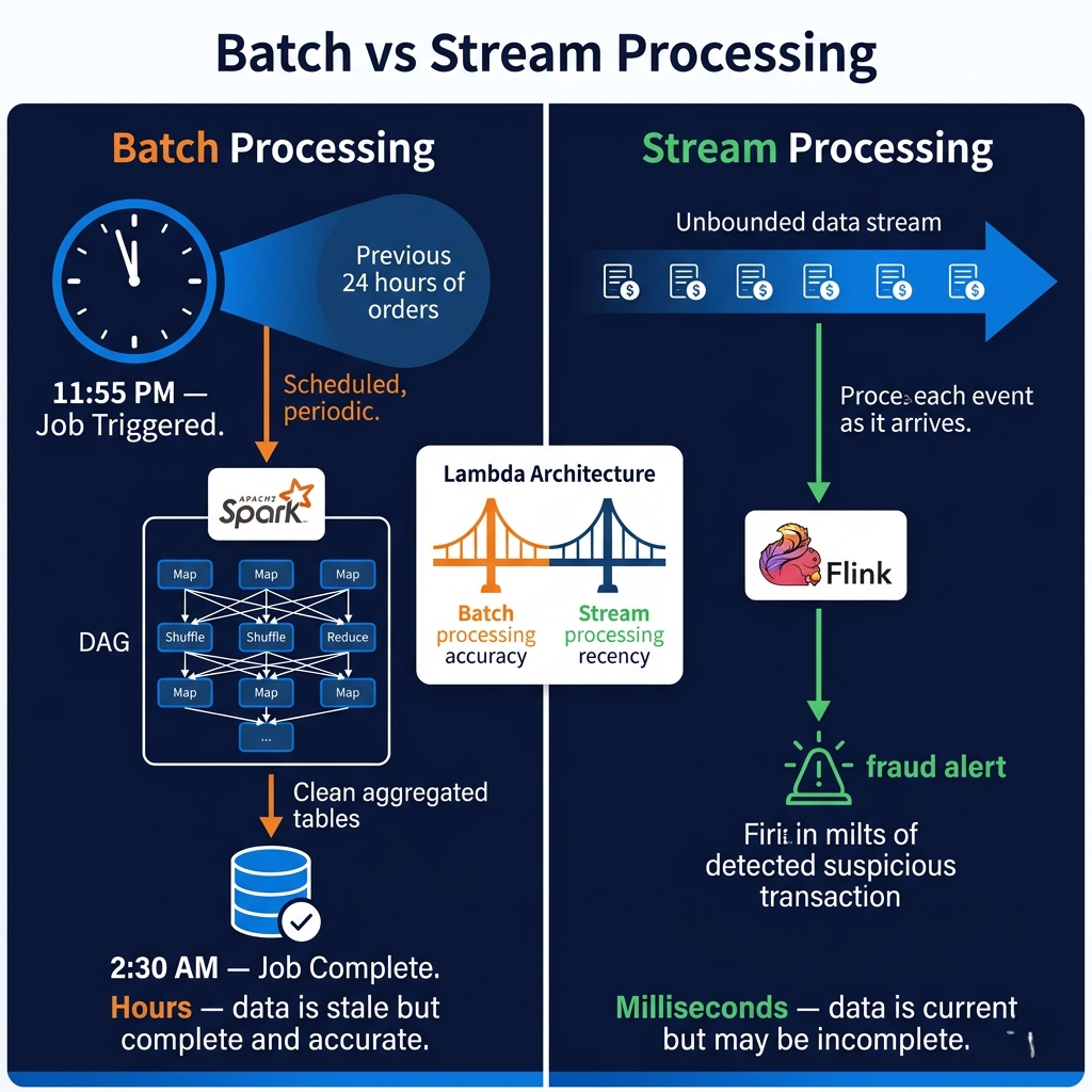
Batch processing operates on bounded datasets — finite collections of data accumulated over a period, processed together in a scheduled job. Apache Spark is the dominant batch processing engine: it distributes computation across a cluster of machines, reads from distributed storage (S3, HDFS), applies transformations through a DAG of operations, and writes results to your data warehouse or data lake. A typical pattern is nightly Spark jobs that aggregate the previous day's transactions, join with user and product data, compute business metrics, and write final tables to Snowflake for the BI team's morning reports. Batch processing excels at complex analytical computations — window functions, joins across multiple large tables, model training on historical datasets — where you have hours to complete the computation and the data completeness of a full batch is more important than recency.
Stream processing operates on unbounded datasets — continuous flows of events processed as they arrive, with latency measured in milliseconds to seconds rather than minutes to hours. Apache Flink is the leading stream processing engine, offering true event-time processing (correctly handling late-arriving events), stateful computation (maintaining running aggregates, session windows, pattern detection state), and exactly-once semantics. A Flink job can detect credit card fraud in real time by analyzing each transaction as it happens, comparing it against a statistical profile of the cardholder's behavior, flagging suspicious patterns, and triggering a review workflow — all before the transaction completes, potentially preventing the fraud rather than just reporting it afterward.
The counterintuitive insight that most introductions to data pipelines miss: batch and stream processing aren't mutually exclusive architectural choices — they're complementary tools for different latency requirements within the same system. A mature data platform uses both: real-time Flink jobs for fraud detection, operational dashboards, and time-sensitive notifications; and nightly Spark jobs for complex historical analytics, model training datasets, and regulatory reporting. The Lambda architecture pattern formalizes this: a speed layer (stream processing for low-latency recent data) and a batch layer (for complete, accurate historical data) with a serving layer that merges results.
# Batch processing with PySpark — nightly sales aggregation
from pyspark.sql import SparkSession
from pyspark.sql import functions as F
from pyspark.sql.types import *
from datetime import datetime, timedelta

spark = SparkSession.builder \
    .appName("nightly-sales-aggregation") \
    .config("spark.sql.extensions", "io.delta.sql.DeltaSparkSessionExtension") \
    .getOrCreate()

# Batch job: process previous day's complete data
processing_date = (datetime.utcnow() - timedelta(days=1)).strftime('%Y-%m-%d')

# Read from S3 data lake (partition pruning makes this fast)
orders_df = spark.read.parquet(f"s3://data-lake/processed/orders/date={processing_date}/")
order_items_df = spark.read.parquet(f"s3://data-lake/processed/order_items/date={processing_date}/")
products_df = spark.read.parquet("s3://data-lake/processed/products/")  # full dimension table

# Complex join and aggregation — batch excels at this
daily_sales = orders_df \
    .filter(F.col('status').isin(['completed', 'delivered'])) \
    .join(order_items_df, 'order_id') \
    .join(products_df, 'product_id') \
    .groupBy('category', 'subcategory', F.col('orders.country').alias('country')) \
    .agg(
        F.count('order_id').alias('order_count'),
        F.sum('total_amount').alias('revenue'),
        F.avg('total_amount').alias('avg_order_value'),
        F.countDistinct('user_id').alias('unique_customers'),
        F.sum(F.when(F.col('is_new_customer'), 1).otherwise(0)).alias('new_customer_orders')
    ) \
    .withColumn('processing_date', F.lit(processing_date)) \
    .withColumn('processed_at', F.current_timestamp())

# Write to data warehouse-ready location (Parquet, partitioned)
daily_sales.write \
    .mode('overwrite') \
    .partitionBy('processing_date') \
    .parquet(f"s3://data-warehouse/sales/daily_by_category/")

print(f"Batch job complete: {daily_sales.count()} category-country combinations processed")
spark.stop()
# Stream processing with Apache Flink (PyFlink) — real-time fraud detection
from pyflink.datastream import StreamExecutionEnvironment
from pyflink.table import StreamTableEnvironment, EnvironmentSettings
from pyflink.table.expressions import col, lit

env = StreamExecutionEnvironment.get_execution_environment()
settings = EnvironmentSettings.new_instance().in_streaming_mode().build()
t_env = StreamTableEnvironment.create(env, environment_settings=settings)

# Define Kafka source — reads transaction events in real time
t_env.execute_sql("""
    CREATE TABLE transactions (
        transaction_id STRING,
        user_id STRING,
        amount DECIMAL(10,2),
        merchant_category STRING,
        country STRING,
        event_time TIMESTAMP(3),
        WATERMARK FOR event_time AS event_time - INTERVAL '5' SECOND
    ) WITH (
        'connector' = 'kafka',
        'topic' = 'payment-transactions',
        'properties.bootstrap.servers' = 'kafka:9092',
        'properties.group.id' = 'fraud-detection-flink',
        'format' = 'json',
        'scan.startup.mode' = 'latest-offset'
    )
""")

# Fraud detection rule: user spending more than 3x their 7-day average in a single transaction
# This runs on every transaction in real time — sub-second latency
t_env.execute_sql("""
    CREATE TABLE fraud_alerts (
        user_id STRING,
        transaction_id STRING,
        amount DECIMAL(10,2),
        seven_day_avg_amount DECIMAL(10,2),
        risk_score DOUBLE,
        alert_time TIMESTAMP(3)
    ) WITH (
        'connector' = 'kafka',
        'topic' = 'fraud-alerts',
        'properties.bootstrap.servers' = 'kafka:9092',
        'format' = 'json'
    )
""")

# Sliding window aggregate + real-time scoring
t_env.execute_sql("""
    INSERT INTO fraud_alerts
    SELECT
        t.user_id,
        t.transaction_id,
        t.amount,
        h.avg_7d_amount,
        CAST(t.amount / NULLIF(h.avg_7d_amount, 0) AS DOUBLE) AS risk_score,
        t.event_time AS alert_time
    FROM transactions t
    JOIN (
        SELECT user_id,
               AVG(amount) AS avg_7d_amount
        FROM transactions
        GROUP BY user_id,
                 TUMBLE(event_time, INTERVAL '1' DAY)
        HAVING COUNT(*) > 5  -- only users with transaction history
    ) h ON t.user_id = h.user_id
    WHERE t.amount > (h.avg_7d_amount * 3)  -- 3x their average = suspicious
      AND t.amount > 500  -- ignore small transactions
""")
Pro Tips & Common Mistakes — Batch vs Stream Processing
Pro Tip: For stream processing, always design for late data. In the real world, events don't arrive in perfect chronological order. A mobile app running in airplane mode records user events locally, then uploads them when connectivity is restored — potentially hours late. Flink's event-time processing with watermarks handles this correctly: process based on when the event actually occurred (event time), not when it arrived at your processor (processing time), and configure a watermark delay that tolerates your expected late-arrival window. Ignoring late data creates phantom gaps in your real-time analytics that look like missing data but are actually just delayed data.
Common Mistake: Using stream processing where batch processing is simpler and sufficient. Real-time streaming adds significant operational complexity: stateful computation that must be checkpointed, exactly-once semantics that require careful configuration, watermark tuning, and distributed state management. If your use case doesn't require sub-minute latency, a well-designed batch job running every 15 minutes is dramatically simpler to build, test, and debug. Streaming is the right tool when you genuinely need real-time — fraud detection, live dashboards, IoT monitoring. It's the wrong tool for "we want our reports faster" when faster means hourly instead of nightly.
ETL and ELT: Transforming Messy Data Into Reliable Structure
Raw data is almost never ready for analysis. It's messy in predictable ways: null values where there shouldn't be any, timestamps in 14 different formats, currency amounts sometimes in cents and sometimes in dollars, customer IDs that should be integers stored as strings, duplicate records from retry logic, and fields with meanings that changed when someone updated the application schema three years ago without telling the data team. The transformation stage is where you turn this chaos into reliable, consistent, queryable structure.
ETL (Extract, Transform, Load) is the traditional approach: extract data from sources, apply transformations in a dedicated compute environment, then load the clean data into the target storage (data warehouse). The transformation happens before the data reaches its final destination, which means your data warehouse only ever contains clean, structured data. Tools like Apache Airflow orchestrate ETL workflows, managing the complex dependencies between extraction jobs, transformation steps, and loading tasks, with scheduling, retries, alerting, and lineage tracking built in. AWS Glue provides a managed ETL service that can auto-discover schema, transform between formats, and load to Redshift or S3 without managing your own Spark cluster.
ELT (Extract, Load, Transform) flips the order: extract from sources, load raw data directly into the data warehouse, then transform within the warehouse using SQL. The rise of cloud data warehouses (Snowflake, BigQuery, Redshift) with massive compute capacity and separation of storage from compute has made ELT increasingly popular. With ELT, your data warehouse stores raw data alongside transformed data; transformations are versioned SQL queries (using tools like dbt — data build tool) that run inside the warehouse. This approach has significant advantages: raw data is always available for debugging and re-transformation, SQL-literate data analysts can write and own transformations without knowing Spark, and the warehouse's query engine handles optimization. The tradeoff is that your warehouse holds (and you pay for storing) raw, potentially sensitive data.
Here's the thing most data engineering guides miss about ETL vs ELT: the choice is less about philosophy and more about your data volume, team skill set, and warehouse capabilities. If your team is SQL-heavy and you're using Snowflake or BigQuery (which scale compute independently of storage), ELT with dbt is often the right choice — it keeps transformations in version control, enables testing with dbt test, and puts transformation ownership closer to the analysts who understand the business logic. If your data is enormous (petabytes), transformations are complex (require Python libraries not available in SQL), or you're working with unstructured data (images, text), ETL with Spark gives you more power and flexibility.
# Apache Airflow DAG — orchestrating an ETL pipeline
# pip install apache-airflow apache-airflow-providers-amazon

from airflow import DAG
from airflow.operators.python import PythonOperator
from airflow.providers.amazon.aws.operators.glue import GlueJobOperator
from airflow.providers.snowflake.operators.snowflake import SnowflakeOperator
from datetime import datetime, timedelta

# DAG definition — the pipeline's blueprint
default_args = {
    'owner': 'data-engineering',
    'depends_on_past': False,
    'email_on_failure': True,
    'email': ['data-alerts@company.com'],
    'retries': 2,
    'retry_delay': timedelta(minutes=5),
    'execution_timeout': timedelta(hours=2)
}

with DAG(
    dag_id='ecommerce_orders_etl',
    description='Daily ETL: extract orders → transform → load to Snowflake',
    schedule_interval='0 2 * * *',  # Run at 2 AM daily
    start_date=datetime(2025, 1, 1),
    catchup=False,
    default_args=default_args,
    tags=['etl', 'orders', 'daily']
) as dag:

    # Task 1: Extract orders from MySQL to S3 staging
    def extract_orders(**context):
        execution_date = context['ds']  # Airflow passes execution date
        orders = collect_from_mysql(last_extracted_at=execution_date)
        result = ingest_batch_to_staging(orders, 'orders', context['run_id'])
        print(f"Extracted: {result.records_ingested}, Rejected: {result.records_rejected}")
        if result.records_rejected > result.records_ingested * 0.01:
            raise ValueError(f"Rejection rate too high: {result.errors[:5]}")
        return result.staging_location

    extract = PythonOperator(
        task_id='extract_orders_from_mysql',
        python_callable=extract_orders
    )

    # Task 2: Transform with AWS Glue (managed Spark)
    transform = GlueJobOperator(
        task_id='transform_orders_with_glue',
        job_name='ecommerce-orders-transformation',
        script_args={
            '--staging_path': "{{ task_instance.xcom_pull(task_ids='extract_orders_from_mysql') }}",
            '--output_path': 's3://data-lake/processed/orders/',
            '--execution_date': '{{ ds }}'
        },
        aws_conn_id='aws_default',
        region_name='us-east-1'
    )

    # Task 3: Load clean data into Snowflake
    load = SnowflakeOperator(
        task_id='load_to_snowflake',
        sql="""
            COPY INTO PROD.ANALYTICS.ORDERS
            FROM @PROD.STAGING.S3_STAGE/processed/orders/date={{ ds }}/
            FILE_FORMAT = (TYPE = 'PARQUET')
            MATCH_BY_COLUMN_NAME = CASE_INSENSITIVE
            ON_ERROR = 'ABORT_STATEMENT';
        """,
        snowflake_conn_id='snowflake_default'
    )

    # Task 4: Validate loaded data
    validate = SnowflakeOperator(
        task_id='validate_loaded_data',
        sql="""
            SELECT CASE
                WHEN COUNT(*) = 0 THEN RAISE_ERROR('No orders loaded for {{ ds }}')
                WHEN COUNT(CASE WHEN order_id IS NULL THEN 1 END) > 0
                    THEN RAISE_ERROR('NULL order_ids found')
                ELSE 'Validation passed: ' || COUNT(*) || ' orders'
            END AS validation_result
            FROM PROD.ANALYTICS.ORDERS
            WHERE DATE(created_at) = '{{ ds }}';
        """
    )

    # DAG dependencies — each task waits for the previous to succeed
    extract >> transform >> load >> validate
-- ELT alternative with dbt — transformations in SQL, inside the warehouse
-- models/staging/stg_orders.sql

{{ config(
    materialized='incremental',
    unique_key='order_id',
    on_schema_change='sync_all_columns'
) }}

SELECT
    -- Normalize ID format (sometimes 'ORD-' prefix, sometimes raw int)
    REGEXP_REPLACE(raw_order_id, '^ORD-', '') AS order_id,

    -- Standardize timestamps (some sources send Unix epoch, some ISO 8601)
    CASE
        WHEN TRY_TO_TIMESTAMP(created_at_raw) IS NOT NULL
            THEN TRY_TO_TIMESTAMP(created_at_raw)
        WHEN TRY_TO_NUMBER(created_at_raw) > 1000000000
            THEN TO_TIMESTAMP(created_at_raw::BIGINT)
        ELSE NULL
    END AS created_at,

    -- Normalize currency amounts (Stripe sends cents, internal DB sends dollars)
    CASE source_system
        WHEN 'stripe' THEN amount_raw / 100.0
        ELSE amount_raw::DECIMAL(10,2)
    END AS total_amount_usd,

    -- Standardize status values (legacy system used 'COMPLETE', new uses 'completed')
    LOWER(REGEXP_REPLACE(status_raw, '[^a-zA-Z_]', '')) AS status,

    COALESCE(customer_id, guest_id) AS user_id,
    country_code,
    _ingested_at,
    CURRENT_TIMESTAMP() AS _transformed_at

FROM {{ source('raw', 'orders') }}

{% if is_incremental() %}
    -- Only process records ingested since last dbt run
    WHERE _ingested_at > (SELECT MAX(_ingested_at) FROM {{ this }})
{% endif %}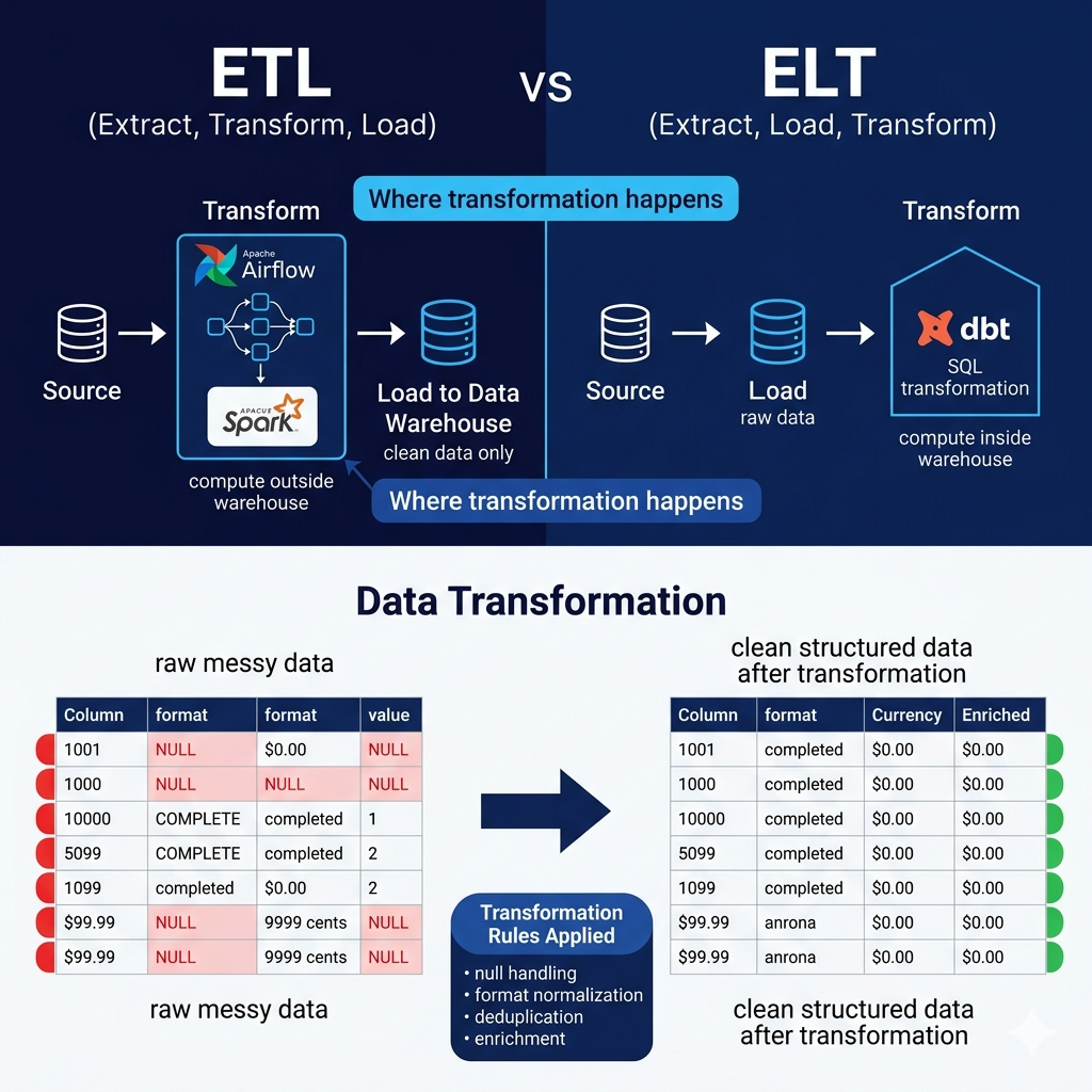
Pro Tips & Common Mistakes — ETL and ELT
Pro Tip: If you're using dbt (and you should seriously consider it for ELT), implement dbt tests from day one — not as an afterthought. dbt's built-in tests (
not_null,unique,accepted_values,relationships) and custom SQL tests serve as a contract for your data quality. Anot_nulltest onorder_idthat fails in CI/CD catches a data quality regression before it corrupts your production analytics. Treat failing dbt tests with the same urgency as failing unit tests in application code — they represent broken contracts with the consumers of your data.
Common Mistake: Putting too much business logic in ETL transformations. Transformations should clean and standardize data — normalize formats, handle nulls, deduplicate records, resolve encoding inconsistencies. They should not implement business rules that change frequently (discount calculations, categorization logic, attribution models). Business logic in ETL jobs is hard to version, hard to test, and painful to change because it requires rerunning historical data. Keep ETL lean and push business logic to the consumption layer (dbt models, BI tool calculations, ML feature engineering) where it's more accessible to the teams that understand it.
Data Storage: Lakes, Warehouses, and Lakehouses
After collection, ingestion, and transformation, data needs a home. The storage layer is where processed data lives until it's consumed by analytics, ML, or other downstream systems — and the choice of storage architecture has profound implications for query performance, storage costs, governance, and the flexibility to support different types of analysis.
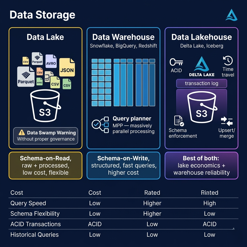
Data lakes store raw and minimally processed data at massive scale using commodity object storage — Amazon S3, Google Cloud Storage, or Azure Blob Storage — with virtually unlimited capacity and extremely low per-GB cost. Data in a data lake is stored in open formats: Parquet (columnar, compressed, efficient for analytical queries), Avro (row-oriented, good for streaming), ORC (highly optimized for Hive workloads), or plain JSON/CSV. The key characteristic of a data lake is schema-on-read: there's no enforced schema when data is stored, only when it's queried. This flexibility is a feature — you can store data before you know exactly how you'll query it — but also a risk: without governance, a data lake quickly becomes a data swamp where nobody knows what's in it, whether it's current, or whether it's reliable.
Data warehouses — Snowflake, Amazon Redshift, Google BigQuery — represent the opposite philosophy: schema-on-write, rigorous structure, optimized for fast analytical SQL queries. Structured data is loaded through defined schemas into column-oriented tables that enable highly efficient aggregation and filtering. A data warehouse can answer "revenue by category by region for the past 90 days" in seconds by scanning only the columns needed (columnar storage), across a massively parallel processing cluster. The tradeoff is cost (warehouses are expensive, especially at scale) and rigidity (you need to know your schema before loading, and schema changes require migration procedures).
Data lakehouses represent the emerging synthesis: technologies like Apache Iceberg, Delta Lake, and Apache Hudi add a transactional metadata layer on top of data lake object storage, providing ACID transactions, schema enforcement, time travel (querying data as it existed at any past point in time), incremental processing support, and efficient updates and deletes — capabilities that object storage lacks natively. A Delta Lake on S3 gives you the storage cost economics of a data lake with many of the reliability and consistency guarantees of a data warehouse. Platforms like Databricks are built on this lakehouse architecture, and cloud providers have been adding native Iceberg support to their warehouse offerings.
# Working with Delta Lake — the lakehouse architecture in practice
# pip install delta-spark pyspark

from pyspark.sql import SparkSession
from delta.tables import DeltaTable
import pyspark.sql.functions as F

spark = SparkSession.builder \
    .appName("lakehouse-demo") \
    .config("spark.sql.extensions", "io.delta.sql.DeltaSparkSessionExtension") \
    .config("spark.sql.catalog.spark_catalog", "org.apache.spark.sql.delta.catalog.DeltaCatalog") \
    .getOrCreate()

DELTA_TABLE_PATH = "s3://data-lake/processed/orders_delta/"

# ============================================================
# UPSERT (MERGE) — Delta Lake supports updates, unlike plain Parquet
# Critical for CDC ingestion: handle updates and deletes correctly
# ============================================================
def upsert_orders(new_orders_df):
    """
    MERGE new/updated orders into the Delta table.
    Plain Parquet can't do this — you'd have to rewrite entire partitions.
    """
    if DeltaTable.isDeltaTable(spark, DELTA_TABLE_PATH):
        delta_table = DeltaTable.forPath(spark, DELTA_TABLE_PATH)
        delta_table.alias("existing") \
            .merge(
                new_orders_df.alias("updates"),
                "existing.order_id = updates.order_id"  # match on primary key
            ) \
            .whenMatchedUpdateAll() \    # UPDATE: replace all fields if order changed
            .whenNotMatchedInsertAll() \ # INSERT: add new orders not yet in table
            .execute()
    else:
        # First write: create the Delta table
        new_orders_df.write.format("delta").save(DELTA_TABLE_PATH)

# ============================================================
# TIME TRAVEL — query data as it existed at a previous point
# Invaluable for debugging "what did this look like before it was wrong?"
# ============================================================

# Query current state
current_orders = spark.read.format("delta").load(DELTA_TABLE_PATH)
print(f"Current order count: {current_orders.count()}")

# Query historical state (e.g., before a bad data load)
orders_yesterday = spark.read \
    .format("delta") \
    .option("timestampAsOf", "2025-01-14 23:59:59") \
    .load(DELTA_TABLE_PATH)
print(f"Yesterday's order count: {orders_yesterday.count()}")

# Query by version number (each write creates a new version)
orders_v5 = spark.read \
    .format("delta") \
    .option("versionAsOf", "5") \
    .load(DELTA_TABLE_PATH)

# ============================================================
# Snowflake — data warehouse consumption layer
# ============================================================
SNOWFLAKE_QUERY = """
-- Analytical query that would crush an OLTP database
-- Data warehouse handles this efficiently with columnar storage + MPP
SELECT
    DATE_TRUNC('month', created_at) AS month,
    country_code,
    product_category,
    COUNT(DISTINCT user_id) AS unique_customers,
    SUM(total_amount_usd) AS revenue,
    AVG(total_amount_usd) AS avg_order_value,
    SUM(SUM(total_amount_usd)) OVER (
        PARTITION BY country_code
        ORDER BY DATE_TRUNC('month', created_at)
    ) AS cumulative_revenue_by_country
FROM PROD.ANALYTICS.ORDERS
WHERE created_at >= '2024-01-01'
  AND status = 'completed'
GROUP BY 1, 2, 3
ORDER BY month DESC, revenue DESC;
"""
Pro Tips & Common Mistakes — Data Storage
Pro Tip: Adopt Apache Iceberg or Delta Lake table format for your data lake storage from the start, not as a migration you'll do "someday." Even if you're not using all their features immediately, these formats give you schema evolution (add columns without rewriting data), partition evolution (change how data is partitioned), time travel, and efficient updates as free capabilities. Migrating from plain Parquet to Iceberg/Delta Lake after your data lake has grown to petabytes is a painful, expensive process. Start with the lakehouse format and never look back.
Common Mistake: Storing everything in a data warehouse and treating storage cost as secondary. Cloud data warehouses charge for compute separately from storage, but storage in structured warehouse tables is still more expensive than S3 object storage. Hot data that's queried frequently belongs in the warehouse. Raw data, historical archives, and infrequently queried datasets belong in the data lake with on-demand query capabilities (Athena, BigQuery external tables, Snowflake external stages). Design your storage tier based on query frequency and latency requirements, not on "put everything in the warehouse because it's easier."
Data Consumption: Turning Data Into Decisions
A data pipeline that stores clean data but doesn't enable good decision-making is infrastructure for its own sake. The consumption layer is where data engineering meets business value — where the processed, structured data in your warehouse becomes insights, predictions, and actions. Understanding how different consumer types work helps you design storage and transformation layers that actually serve their needs.
Business intelligence and dashboards are the broadest consumption pattern. Tools like Tableau, Power BI, and Looker connect directly to data warehouses and lakehouses, enabling non-technical users to build visualizations, slice and dice data, and track KPIs. Looker's LookML — a SQL-based modeling layer — defines business logic (what does "active customer" mean? how is "revenue" calculated?) in a centralized, version-controlled way, so every dashboard using the "revenue" metric uses the same definition. This semantic layer approach prevents the "which number is right?" problem that plagues organizations where every team has their own revenue calculation in their own spreadsheet.
Data science and machine learning consume data at a different layer. ML models typically need large volumes of historical data in formats optimized for training (feature tables, label datasets, time-series sequences). Data scientists access this data through notebooks (Jupyter, Databricks notebooks) connected to the data warehouse or data lake, with Python libraries like Pandas, scikit-learn, TensorFlow, and PyTorch for model training. A customer churn model needs a training dataset joining user activity from the event stream, transaction history from the warehouse, support ticket data from the CRM, and product usage metrics from the application database — exactly the kind of multi-source join that a data pipeline makes possible at scale.
Machine learning in production requires not just historical data but continuous data feeds for ongoing model retraining and real-time inference. A fraud detection model trained on last month's data may be obsolete today as fraud patterns evolve. Continuous training pipelines regularly ingest new labeled data, retrain models, evaluate performance, and deploy updated models — all automated. Feature stores (Feast, Tecton, AWS SageMaker Feature Store) bridge the offline training world and the online inference world, making features computed from your batch pipeline available for real-time ML inference with low latency.
# Complete consumption layer examples

# ============================================================
# 1. Self-serve analytics with pandas + Snowflake connector
# ============================================================
import snowflake.connector
import pandas as pd
import matplotlib.pyplot as plt

def get_monthly_revenue_by_segment(start_date: str, end_date: str) -> pd.DataFrame:
    """Data scientist / analyst self-service query pattern."""
    conn = snowflake.connector.connect(
        account='company.snowflakecomputing.com',
        user='analyst@company.com',
        authenticator='externalbrowser',  # SSO authentication
        warehouse='ANALYTICS_WH',
        database='PROD',
        schema='ANALYTICS'
    )
    query = f"""
        SELECT
            DATE_TRUNC('month', o.created_at) AS month,
            c.customer_segment,
            SUM(o.total_amount_usd) AS revenue,
            COUNT(DISTINCT o.user_id) AS customers
        FROM ORDERS o
        JOIN CUSTOMERS c USING (user_id)
        WHERE o.created_at BETWEEN '{start_date}' AND '{end_date}'
          AND o.status = 'completed'
        GROUP BY 1, 2
        ORDER BY 1, 4 DESC
    """
    return pd.read_sql(query, conn)

df = get_monthly_revenue_by_segment('2024-01-01', '2024-12-31')
df.pivot(index='month', columns='customer_segment', values='revenue').plot(kind='bar')


# ============================================================
# 2. ML feature engineering for churn prediction
# ============================================================
from sklearn.ensemble import GradientBoostingClassifier
from sklearn.model_selection import train_test_split
from sklearn.preprocessing import StandardScaler
import numpy as np

def build_churn_features(user_ids: list, reference_date: str) -> pd.DataFrame:
    """
    Build feature table for churn prediction from the data warehouse.
    Features computed from the last 90 days of activity.
    """
    conn = snowflake.connector.connect(...)
    feature_query = f"""
        SELECT
            u.user_id,
            -- Recency features
            DATEDIFF('day', MAX(o.created_at), '{reference_date}') AS days_since_last_order,
            DATEDIFF('day', MIN(o.created_at), '{reference_date}') AS days_since_first_order,

            -- Frequency features
            COUNT(o.order_id) AS total_orders_90d,
            COUNT(DISTINCT DATE_TRUNC('week', o.created_at)) AS active_weeks_90d,

            -- Monetary features
            SUM(o.total_amount_usd) AS total_spend_90d,
            AVG(o.total_amount_usd) AS avg_order_value_90d,

            -- Engagement features
            COUNT(DISTINCT e.session_id) AS sessions_90d,
            SUM(CASE WHEN e.event_type = 'search' THEN 1 ELSE 0 END) AS search_count_90d,

            -- Target variable: churned = no purchase in last 30 days
            CASE WHEN MAX(o.created_at) < DATEADD('day', -30, '{reference_date}')
                 THEN 1 ELSE 0 END AS churned
        FROM USERS u
        LEFT JOIN ORDERS o ON u.user_id = o.user_id
            AND o.created_at >= DATEADD('day', -90, '{reference_date}')
        LEFT JOIN USER_EVENTS e ON u.user_id = e.user_id
            AND e.event_time >= DATEADD('day', -90, '{reference_date}')
        WHERE u.user_id IN ({','.join(f"'{uid}'" for uid in user_ids)})
        GROUP BY 1
    """
    return pd.read_sql(feature_query, conn)

# Train churn model
features_df = build_churn_features(user_ids=[...], reference_date='2024-12-01')
feature_cols = [c for c in features_df.columns if c not in ['user_id', 'churned']]

X = features_df[feature_cols].fillna(0)
y = features_df['churned']
X_train, X_test, y_train, y_test = train_test_split(X, y, test_size=0.2, random_state=42)

scaler = StandardScaler()
model = GradientBoostingClassifier(n_estimators=200, max_depth=4)
model.fit(scaler.fit_transform(X_train), y_train)

# Feature importance — which signals most predict churn?
for feature, importance in sorted(
    zip(feature_cols, model.feature_importances_),
    key=lambda x: x[1], reverse=True
)[:5]:
    print(f"{feature}: {importance:.3f}")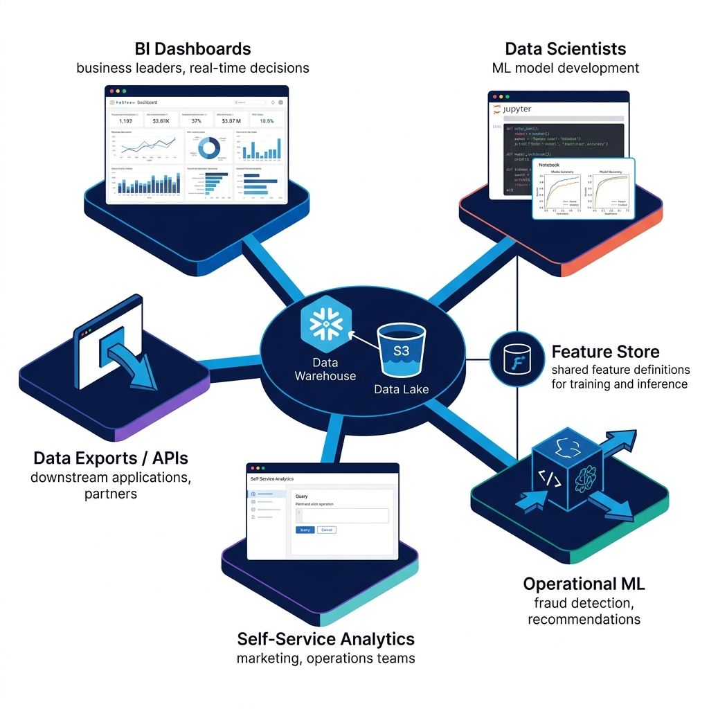
Pro Tips & Common Mistakes — Data Consumption
Pro Tip: Build a semantic layer (using Looker's LookML, dbt metrics, or a dedicated tool like Cube.dev) to define business metrics centrally and consistently. "Revenue," "active user," "conversion rate" — these terms mean different things to different teams without a canonical definition. A semantic layer defines these metrics once, enforces consistent calculation across all BI tools and queries, and prevents the proliferation of contradictory metrics that erode trust in data. When the CEO's dashboard and the VP's report show different numbers for "monthly revenue," the problem is almost always a missing or ignored semantic layer.
Common Mistake: Giving data scientists direct write access to production data warehouse tables "temporarily" for exploration. Exploratory analysis that mutates production tables (even accidentally) causes data quality incidents that cascade across every dashboard and model relying on those tables. Provide data scientists with a dedicated sandbox schema or environment where they have full write access, and enforce strict read-only access to production tables. Make the sandbox easy to use and provision self-service; engineers will only bypass security controls when they're more inconvenient than the risk they're protecting against.
How It All Connects: The Complete Data Pipeline Architecture
Walking through the five stages reveals how they form a coherent system rather than isolated components. Data originates in operational systems — transactional databases, event streams, application logs, external APIs — each source generating data continuously at its own rate and in its own format. Collection is the act of reaching into these diverse sources and acquiring the data; ingestion is loading it into the pipeline environment, typically through Kafka for streams (CDC-based or direct event publication) and S3 staging for batch data.
The compute stage applies intelligence to raw data. Batch processing (Spark) handles the complex historical analytics and model training datasets that don't need real-time results. Stream processing (Flink) handles fraud detection, real-time dashboards, and event-driven workflows that do. ETL and ELT transformations clean, normalize, and enrich data — making it reliable and consistent enough to build decisions on. The quality of these transformations directly determines the quality of every downstream insight.
Transformed data lands in the storage layer — a lake for raw and semi-processed data, a warehouse for structured analytical queries, a lakehouse for systems that need both. From storage, data flows to consumers: BI tools for business reporting, data scientists for model development, ML systems for real-time inference, and operational teams for self-service analysis. The entire architecture is only as strong as its weakest stage — a perfect storage layer is worthless if the transformation stage is silently corrupting data, and a perfect transformation is useless if the collection stage is missing 30% of events.
The critical insight that unifies all five stages: a data pipeline is not a set of tools — it's an operating contract. Every stage makes promises to the stage downstream: "I'll deliver all events with no losses." "I'll clean this data according to these rules." "I'll make this query available within this SLA." When those contracts are broken — silently, at 3 a.m., because a CDC connector lost its database connection or a Spark job failed on its fourth retry without alerting anyone — the data that downstream teams trusted becomes lies dressed up as facts. Monitoring, alerting, data quality checks, and SLA enforcement are what turn a collection of tools into a trustworthy data pipeline.
Getting Started: Building Your First Data Pipeline
Here's a practical path from zero to a working end-to-end data pipeline using open-source tools.
Step 1: Set up the local infrastructure
# Docker Compose for local development stack
# Save as docker-compose.yml

cat > docker-compose.yml << 'EOF'
version: '3.8'
services:
  postgres:
    image: postgres:15
    environment:
      POSTGRES_DB: ecommerce
      POSTGRES_USER: pipeline
      POSTGRES_PASSWORD: pipeline123
    ports: ["5432:5432"]
    command: ["postgres", "-c", "wal_level=logical"]  # enable CDC

  kafka:
    image: confluentinc/cp-kafka:7.5.0
    depends_on: [zookeeper]
    ports: ["9092:9092"]
    environment:
      KAFKA_ZOOKEEPER_CONNECT: zookeeper:2181
      KAFKA_ADVERTISED_LISTENERS: PLAINTEXT://localhost:9092
      KAFKA_AUTO_CREATE_TOPICS_ENABLE: "true"

  zookeeper:
    image: confluentinc/cp-zookeeper:7.5.0
    environment:
      ZOOKEEPER_CLIENT_PORT: 2181

  airflow:
    image: apache/airflow:2.8.0
    ports: ["8080:8080"]
    environment:
      AIRFLOW__CORE__EXECUTOR: LocalExecutor
      AIRFLOW__DATABASE__SQL_ALCHEMY_CONN: postgresql+psycopg2://pipeline:pipeline123@postgres/airflow
    command: standalone
    volumes:
      - ./dags:/opt/airflow/dags
      - ./logs:/opt/airflow/logs

  minio:  # S3-compatible local object storage
    image: minio/minio:latest
    ports: ["9000:9000", "9001:9001"]
    environment:
      MINIO_ROOT_USER: minioadmin
      MINIO_ROOT_PASSWORD: minioadmin
    command: server /data --console-address ":9001"
EOF

docker-compose up -d
Step 2: Create a simple batch pipeline DAG
# dags/simple_orders_pipeline.py
from airflow import DAG
from airflow.operators.python import PythonOperator
from datetime import datetime, timedelta
import psycopg2
import pandas as pd
import boto3
import json

def extract_orders(**context):
    """Extract orders from PostgreSQL."""
    conn = psycopg2.connect("host=postgres dbname=ecommerce user=pipeline password=pipeline123")
    df = pd.read_sql(
        "SELECT * FROM orders WHERE created_at::date = %s",
        conn, params=[context['ds']]
    )
    # Stage raw data in MinIO (local S3)
    s3 = boto3.client('s3', endpoint_url='http://minio:9000',
                      aws_access_key_id='minioadmin', aws_secret_access_key='minioadmin')
    s3.put_object(
        Bucket='data-lake',
        Key=f"raw/orders/{context['ds']}/data.json",
        Body=df.to_json(orient='records').encode()
    )
    return len(df)

def transform_orders(**context):
    """Clean and transform staged orders."""
    s3 = boto3.client('s3', endpoint_url='http://minio:9000',
                      aws_access_key_id='minioadmin', aws_secret_access_key='minioadmin')
    raw = json.loads(s3.get_object(Bucket='data-lake',
                     Key=f"raw/orders/{context['ds']}/data.json")['Body'].read())
    df = pd.DataFrame(raw)

    # Transformations
    df['total_amount'] = df['total_amount'].abs()  # fix negative amounts from refunds
    df['status'] = df['status'].str.lower().str.strip()  # normalize status
    df = df.dropna(subset=['order_id', 'user_id'])  # drop records with null PKs
    df['_transformed_at'] = datetime.utcnow().isoformat()

    s3.put_object(
        Bucket='data-lake',
        Key=f"processed/orders/{context['ds']}/data.json",
        Body=df.to_json(orient='records').encode()
    )

with DAG('simple_orders_pipeline', schedule_interval='@daily',
         start_date=datetime(2025, 1, 1), catchup=False) as dag:
    extract = PythonOperator(task_id='extract', python_callable=extract_orders)
    transform = PythonOperator(task_id='transform', python_callable=transform_orders)

    extract >> transform
Step 3: Add data quality checks
# Great Expectations for data validation
pip install great-expectations

# Create expectations for your orders data
import great_expectations as gx

context = gx.get_context()
datasource = context.sources.add_pandas("orders_source")
asset = datasource.add_csv_asset("orders", filepath_or_buffer="orders.csv")
batch = asset.get_batch_request()

validator = context.get_validator(batch_request=batch)
validator.expect_column_values_to_not_be_null("order_id")
validator.expect_column_values_to_be_unique("order_id")
validator.expect_column_values_to_be_between("total_amount", min_value=0, max_value=100000)
validator.expect_column_values_to_be_in_set("status",
    ["pending", "completed", "cancelled", "refunded"])

results = validator.validate()
if not results["success"]:
    raise ValueError(f"Data quality checks failed: {results['statistics']}")
print(f"Quality check passed: {results['statistics']['successful_expectations']} checks")
Step 4: Set up monitoring
# Key metrics to monitor for each pipeline stage:

# 1. Kafka consumer lag (ingestion health)
docker exec kafka kafka-consumer-groups \
  --bootstrap-server localhost:9092 \
  --group your-ingestion-group --describe

# 2. Airflow DAG run status (pipeline execution health)
# Airflow UI at http://localhost:8080
# Look for: DAG run status, task duration trends, failure counts

# 3. Data freshness check (is data arriving on time?)
# Run in your data warehouse:
SELECT
  MAX(created_at) AS latest_record,
  DATEDIFF('minute', MAX(created_at), CURRENT_TIMESTAMP()) AS minutes_stale,
  CASE WHEN DATEDIFF('minute', MAX(created_at), CURRENT_TIMESTAMP()) > 60
       THEN 'ALERT: Data is stale'
       ELSE 'OK' END AS status
FROM orders;
FAQ
Q: What is a data pipeline and how does it work?
A data pipeline is an automated system that moves data from its sources (databases, event streams, APIs) through stages of processing and transformation to a destination where it can be analyzed and acted upon. The pipeline handles collection (acquiring raw data), ingestion (loading it into the pipeline environment), computation (batch or stream processing, ETL/ELT transformations), storage (data lakes, warehouses, or lakehouses), and consumption (BI dashboards, ML models, self-service analytics). Pipelines automate what would otherwise be manual data preparation, enabling consistent, reliable, scalable data flows that power business decisions.
Q: What is the difference between ETL and ELT?
ETL (Extract, Transform, Load) transforms data before loading it into the destination storage — transformation happens in a dedicated compute environment (Apache Spark, AWS Glue) and only clean data reaches the warehouse. ELT (Extract, Load, Transform) loads raw data into the warehouse first, then transforms it inside the warehouse using SQL (commonly with dbt). ELT has become more popular with powerful cloud data warehouses (Snowflake, BigQuery) because it keeps raw data available for reprocessing, allows analysts to own transformations in SQL, and leverages the warehouse's compute power. ETL remains relevant for complex transformations requiring Python code, very large datasets, or unstructured data.
Q: What is the difference between batch processing and stream processing?
Batch processing operates on bounded datasets — accumulating data over a period, then processing all of it in a scheduled job. Apache Spark is the dominant batch engine. It excels at complex historical analytics, model training, and large-scale joins where completeness matters more than recency (nightly reports, monthly summaries). Stream processing operates on unbounded, continuous data flows, processing events as they arrive with millisecond to second latency. Apache Flink is the leading stream engine. It excels at real-time fraud detection, live dashboards, alerting, and event-driven systems where timeliness matters more than completeness. Most mature data platforms use both.
Q: What is a data lake versus a data warehouse?
A data lake stores raw and minimally processed data in open formats (Parquet, JSON, CSV) in object storage (S3) with schema defined at query time — flexible, cheap, but requires governance to avoid becoming a disorganized "data swamp." A data warehouse (Snowflake, BigQuery, Redshift) stores structured, transformed data in column-oriented tables with predefined schemas, optimized for fast analytical SQL queries — more expensive but faster and more reliable for querying. A data lakehouse (using Delta Lake or Apache Iceberg) combines both: lake-scale object storage with warehouse-like ACID transactions, schema enforcement, and time travel.
Q: What tools are used in data pipelines?
Data pipeline tools span every stage. For ingestion: Apache Kafka, Amazon Kinesis, Debezium. For batch processing: Apache Spark, Apache Hive, AWS Glue. For stream processing: Apache Flink, Google Cloud Dataflow, Apache Storm. For orchestration (scheduling and managing pipeline workflows): Apache Airflow, Prefect, Dagster. For transformation: dbt (data build tool), Apache Spark, AWS Glue. For storage: Amazon S3, Apache Parquet format, Snowflake, Google BigQuery, Amazon Redshift, Delta Lake, Apache Iceberg. For consumption: Tableau, Power BI, Looker, Jupyter Notebooks, TensorFlow/PyTorch.
Q: How do I handle data quality in a data pipeline?
Data quality requires checks at multiple stages. At ingestion, validate that required fields are present and data types match expectations before writing to staging. In transformation, apply normalization, handle nulls, deduplicate records, and validate referential integrity. At the storage layer, use tools like Great Expectations or dbt tests to run automated quality checks (not_null, unique, value range, referential integrity) as part of your pipeline. At the consumption layer, implement freshness checks (how old is the most recent data?) and row count checks (are we seeing expected volumes?). Set up alerting for quality check failures and treat them with the same urgency as production application failures.
Q: What is Change Data Capture (CDC) and when should I use it?
CDC captures row-level changes (inserts, updates, deletes) from a database's transaction log rather than querying the database directly. Tools like Debezium tap into MySQL's binary log, PostgreSQL's WAL, or MongoDB's oplog and publish change events to Kafka in real time. Use CDC when you need to capture deletes (timestamp-based polling can't detect deleted rows), need real-time data propagation rather than periodic batch extraction, have tables without reliable updated_at timestamps, or need to minimize load on source production databases. CDC is the modern standard for database ingestion in data pipelines and is significantly more reliable than polling-based approaches.
Conclusion
Netflix's recommendation engine problem from this post's opening wasn't solved by building a better ML model. It was solved by building a better data pipeline — one with proper monitoring, real-time event stream integration, and the reliability guarantees that let the ML team trust the data feeding their models. The pipeline became invisible in the best possible way: it worked, consistently, so the data team could focus on the interesting problems instead of debugging why yesterday's numbers are wrong.
That invisibility is the goal of good data pipeline engineering. When a pipeline is working well, nobody thinks about it — business analysts get fresh data in their dashboards, ML models get training data that reflects current patterns, executives see accurate KPIs. When a pipeline is working poorly, everyone thinks about it — data is stale, numbers contradict each other, the data team spends more time debugging pipelines than doing analysis, and trust in data erodes.
The five stages covered here — collect, ingest, compute, store, consume — aren't just a framework for understanding existing pipelines. They're a checklist for evaluating whether a pipeline you're building or inheriting is actually reliable. Is collection incremental and monitored? Is ingestion staging raw data for replay? Is the compute layer handling late data and failures gracefully? Is the storage layer optimized for actual query patterns? Is the consumption layer built on a semantic layer that prevents metric definitions from fracturing? A "yes" to each question is the difference between a data asset and a liability.