A junior engineer once asked me why their search feature worked perfectly in staging and fell apart in production. The code was identical. The logic was sound. The tests all passed. But with 2 million users in the database instead of 200 test records, the endpoint started timing out.

The answer was a nested loop — two for loops, one inside the other, iterating over the same dataset to find matching records. At 200 rows, it ran in milliseconds. At 2 million rows, it would theoretically take longer than anyone would wait. The code wasn't broken. It was just blind to scale. And the engineer had never been taught the vocabulary to see the problem coming.

That vocabulary is Big O Notation. It's the language engineers use to describe how an algorithm's runtime or memory usage grows as the input grows. It's what separates "this works" from "this works at any scale." It's the difference between a search that handles 200 users and one that handles 200 million. And despite what the textbooks make you think, it's not nearly as intimidating once someone explains it like a human being — which is exactly what this post is going to do.

Table of Contents

1. What Big O Notation Actually Means
2. O(1) — Constant Time: The Holy Grail
3. O(log n) — Logarithmic Time: The Efficient Eliminator
4. O(n) — Linear Time: The Honest Workhorse
5. O(n log n) — Linearithmic Time: Where Sorting Lives
6. O(n²) and Beyond: The Danger Zone
7. The Hardware Truth: Why Big O Is Only Half the Story
8. How It All Connects: Reading Complexity Like a Senior Engineer
9. Getting Started: Analyzing Your Own Code
10. FAQ
11. Conclusion

What Big O Notation Actually Means 

Before we look at any specific notation, let's get the mental model right — because most explanations start with math and lose you before the useful part.

Big O Notation is a way of describing how an algorithm scales. Not how fast it runs on your machine right now. Not how many milliseconds it takes. It's about the shape of the growth curve as the input size (called n) gets larger. If you double your input, does the runtime stay the same? Double? Quadruple? Explode exponentially? Big O answers that question with a single, hardware-agnostic expression.

The "O" stands for "Order of," and the notation describes the upper bound of growth — the worst case behavior you can expect. O(n) means: in the worst case, if you have n inputs, you'll do roughly n operations. The constants are stripped out because what we care about at scale is the dominant term. An algorithm that does 3n + 50 operations is still O(n) — when n is 10 million, that constant 50 is noise. The 3n is what matters, and even the 3 gets dropped because we're describing growth shape, not raw speed.

Here's the thing most tutorials miss when they introduce Big O: it's a design tool, not a grading system. The goal isn't to achieve the lowest Big O class at all costs — it's to understand the tradeoffs you're making so you can make informed decisions. A perfectly valid system might use an O(n²) algorithm on purpose, because the input is always small, or because the constant factors of a "better" algorithm make it slower in practice. Big O gives you the vocabulary to have that conversation intelligently.

The common notations, ranked fastest to slowest by growth rate: O(1), O(log n), O(n), O(n log n), O(n²), O(n³), O(2^n), O(n!). Let's walk through each one like it actually matters in production — because it does.

Pro Tips & Common Mistakes — Understanding Big O

Pro Tip: When analyzing your own code, a quick shortcut is to count your loop nesting depth. One loop = O(n). Two nested loops = O(n²). Three nested loops = O(n³). This isn't always exact, but it catches 90% of complexity problems in real code.

Common Mistake: Confusing time complexity with actual execution speed. An O(n log n) sort on 1,000 items might run in 0.1ms. An O(1) hash lookup with a terrible hash function might take 50ms. Big O describes scaling behavior — profiling tells you actual speed. Use both.

Myth-busted: "I should always use the algorithm with the lowest Big O." Not true. For small inputs, an O(n²) algorithm with a tiny constant can outperform an O(n log n) algorithm with large overhead. Python's sort() uses Timsort, which exploits real-world patterns in data to be faster in practice than its worst-case O(n log n) suggests.

O(1) — Constant Time: The Holy Grail 

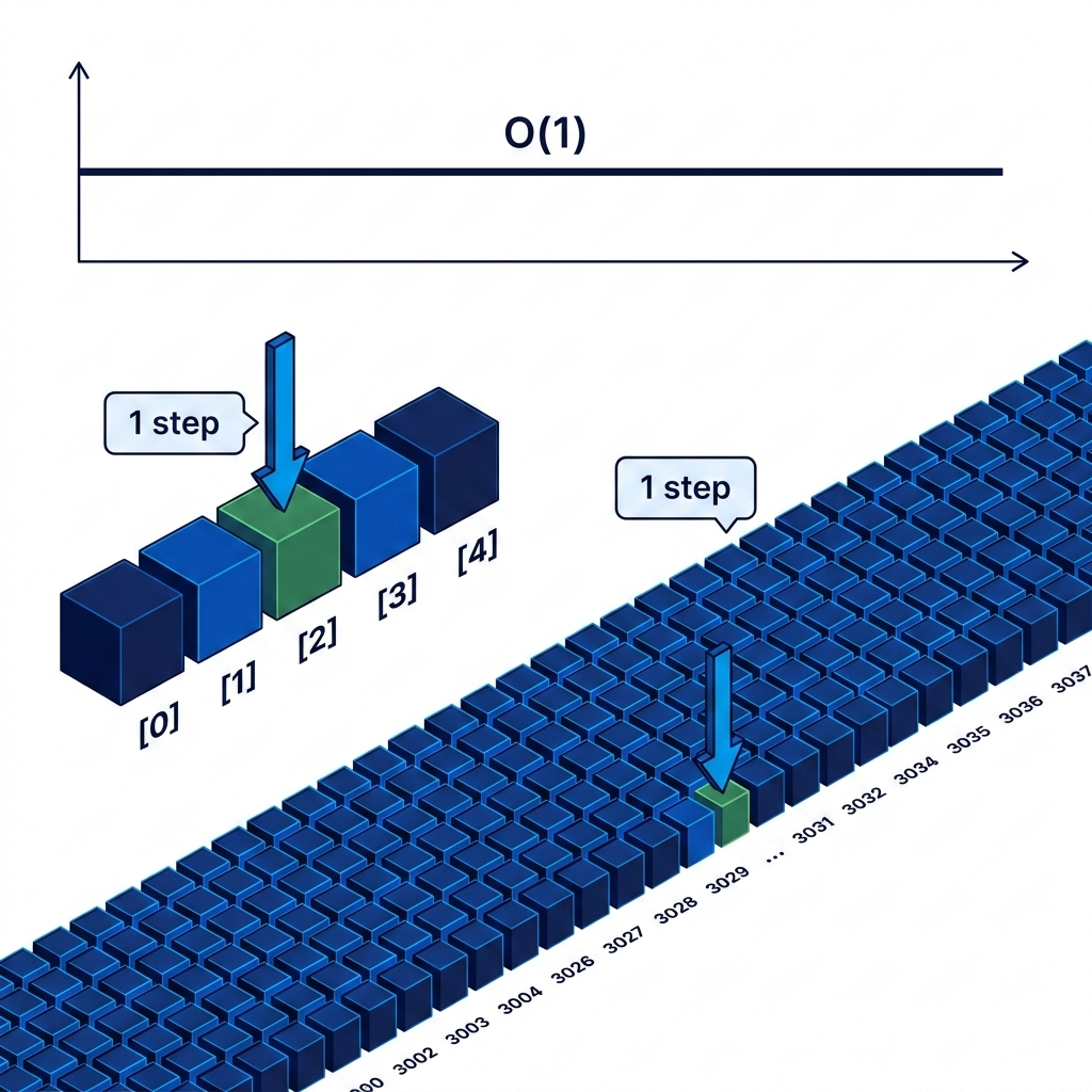
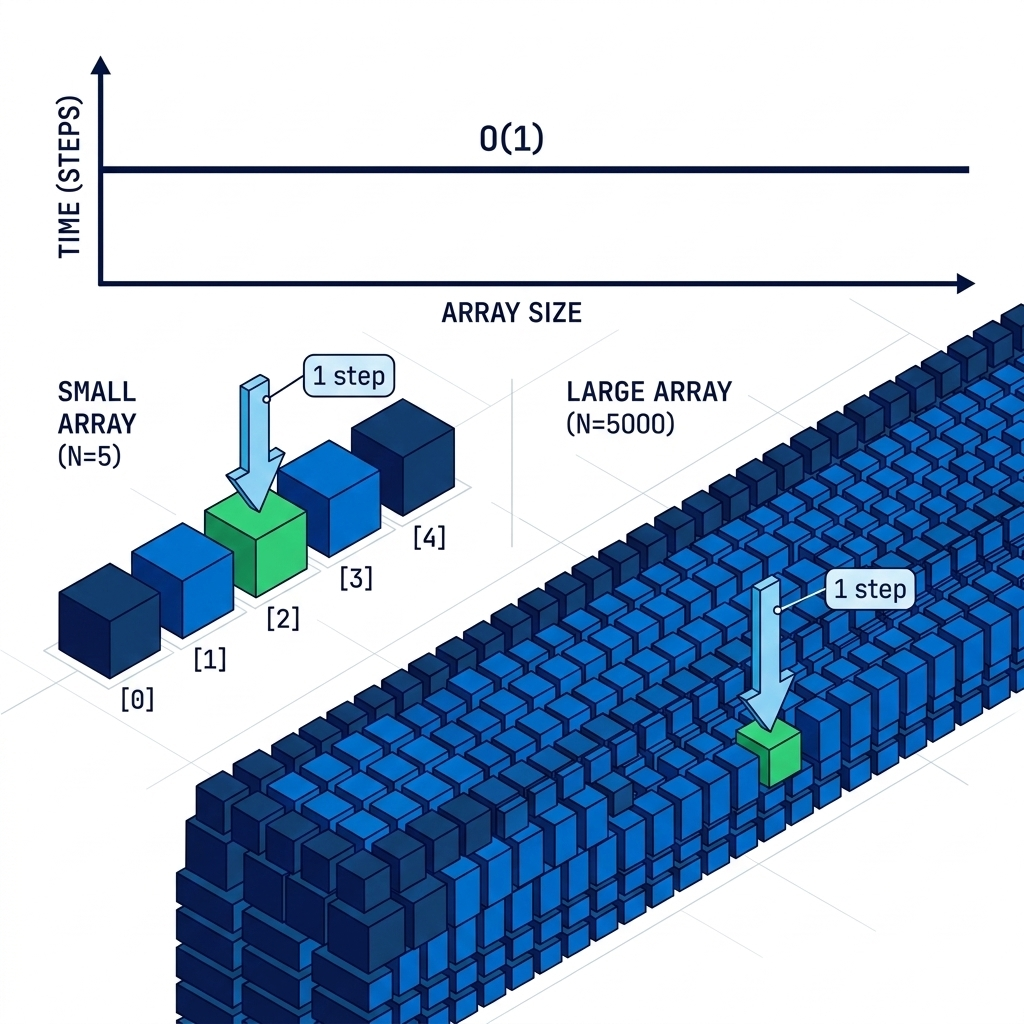
O(1) means the operation takes the same amount of time no matter how large the input is. You have 10 items or 10 billion items — the operation completes in the same number of steps. This is the performance ceiling every engineer is chasing.

The canonical example is array index access. When you write myArray[42], the computer doesn't scan through 42 elements to find the 43rd — it calculates the memory address directly using the base address plus the index times the element size, then reads from that address in a single operation. No searching. No iterating. One jump. This works because arrays store data in contiguous memory blocks, so the math is trivially cheap.

Hash tables are the other O(1) superstar. Lookups, insertions, and deletions in a hash table are constant time on average — meaning checking whether a username already exists in a database of 500 million users takes the same time as checking in a database of 5 users. This is why hash tables (dictionaries in Python, objects in JavaScript, HashMaps in Java) are so pervasive in high-performance code. Any time you see an engineer replace a for loop search with a lookup in a pre-built dictionary, you're watching someone convert O(n) work into O(1) work.

# O(n) approach — scanning a list to check membership
def has_permission_slow(user_id, allowed_users_list):
    for user in allowed_users_list:  # scans every item
        if user == user_id:
            return True
    return False

# O(1) approach — hash set lookup
def has_permission_fast(user_id, allowed_users_set):
    return user_id in allowed_users_set  # direct hash lookup, ~constant time

# The difference at scale:
# allowed_users_list with 1,000,000 users → up to 1,000,000 comparisons
# allowed_users_set with 1,000,000 users  → ~1 comparison
allowed_set = set(allowed_users_list)  # one-time O(n) conversion

Pro Tips & Common Mistakes — O(1)

Pro Tip: Hash table lookups are O(1) on average, not always. In the worst case (when many keys hash to the same bucket — called a collision), lookup degrades to O(n). Python's dict and set implementations handle this well, but if you're building a hash table from scratch or working in a security-sensitive context, be aware of hash flooding attacks that deliberately trigger worst-case behavior.

Common Mistake: Assuming "O(1)" means "instant." Constant time just means the runtime doesn't scale with input size. The constant itself can still be large. A Redis lookup is O(1) but involves a network round-trip — which might be 1ms. That's fine for most things, but it adds up if you're making 10,000 Redis calls in a single request.

O(log n) — Logarithmic Time: The Efficient Eliminator

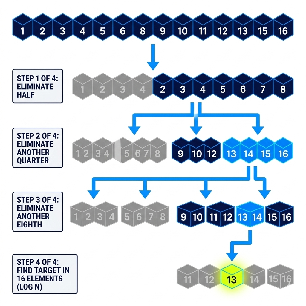
O(log n) is the complexity class that feels like magic once you understand it. Logarithmic algorithms get dramatically more efficient relative to their input as the input grows — because each step eliminates not one element but half of all remaining possibilities.

The textbook example is binary search. Imagine you're looking up a word in a physical dictionary. You don't start from page 1 and read every entry. You open to the middle, check whether your word comes before or after that page, then open to the middle of the relevant half. You've just eliminated 50% of the dictionary in one step. Do it again — another 50% gone. Binary search on a sorted array of 1 million elements finds its target in at most 20 steps. That's log₂(1,000,000) ≈ 20. Compare that to linear search, which might take 1,000,000 steps in the worst case.

The reason this matters so deeply in practice is that many foundational data structures rely on logarithmic operations. Binary search trees, balanced BSTs (like AVL trees and red-black trees), and B-trees (which power database indexes) all offer O(log n) insertion, deletion, and lookup. When your database can find a row among 50 million records in a handful of comparisons rather than a full table scan, that's O(log n) at work in the form of a B-tree index.

# Binary search — O(log n) on a sorted array
def binary_search(arr, target):
    left, right = 0, len(arr) - 1

    while left <= right:
        mid = (left + right) // 2  # find the middle

        if arr[mid] == target:
            return mid              # found it
        elif arr[mid] < target:
            left = mid + 1          # eliminate left half
        else:
            right = mid - 1         # eliminate right half

    return -1  # not found

# At scale:
# Linear search in 1,000,000 items: up to 1,000,000 comparisons
# Binary search in 1,000,000 items: at most 20 comparisons
# Binary search in 1,000,000,000 items: at most 30 comparisons

sorted_data = list(range(1_000_000))
result = binary_search(sorted_data, 847_293)  # ~20 steps, not 847,293

The key insight about O(log n) is how slowly it grows. Doubling the input size adds only one extra step. Going from 1 million to 1 billion items (a 1000x increase in data) only adds 10 more steps to a binary search. That's the power of halving — it turns massive scale problems into trivially small ones.

Pro Tips & Common Mistakes — O(log n)

Pro Tip: Binary search only works on sorted data. The most common mistake is applying binary search to an unsorted collection and getting wrong answers with no error — the algorithm runs, produces an output, and the output is silently incorrect. Always verify your data is sorted before using binary search, or use a data structure (like a sorted set or BST) that maintains sort order automatically.

Common Mistake: Forgetting that database query performance is O(log n) with an index and O(n) without one. Adding the right index to a slow query is one of the highest-leverage performance improvements you can make. A query that scans 10 million rows without an index versus one that uses a B-tree index to find a record in ~23 comparisons is the difference between a 10-second response and a 2ms response.

O(n) — Linear Time: The Honest Workhorse 

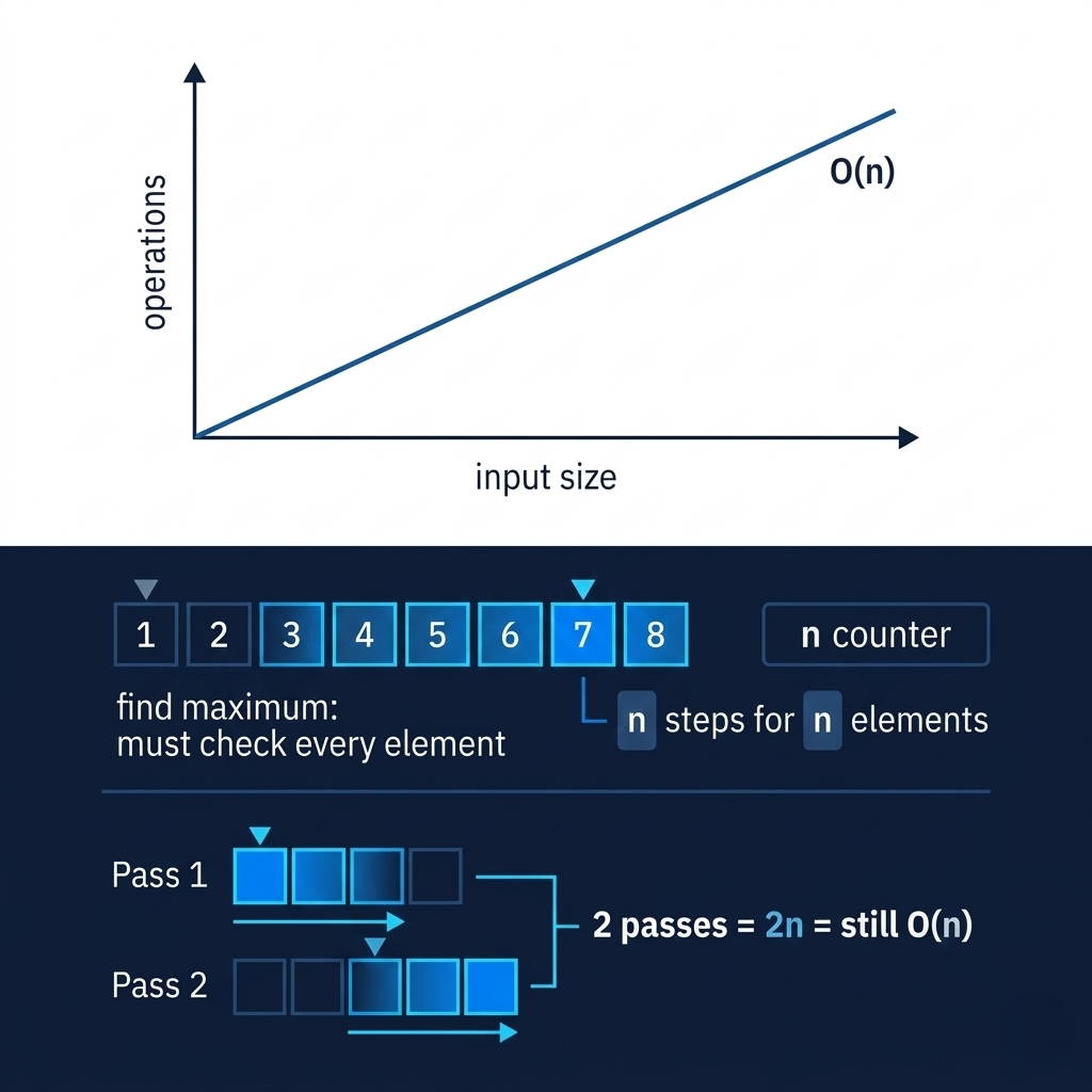
O(n) is the baseline of "sensible." The runtime grows directly in proportion to the input size — twice as many items, twice as long. It's not the fastest, but it's completely predictable and often unavoidable.

The simplest example is finding the maximum value in an unsorted array. You have no choice but to look at every element — there's no shortcut, no binary search you can apply without sorting first. This is O(n): one pass through the data, one comparison per element. When you reach the end, you have your answer. It's honest work.

Most data processing you do is inherently O(n). Reading a file line by line is O(n). Applying a transformation to every item in a list is O(n). Counting occurrences of a word across a document is O(n). This is the complexity class that says "I need to touch every piece of data at least once," and that's often completely reasonable and correct. The goal isn't to avoid O(n) — it's to avoid accidentally going beyond it when you don't have to.

# O(n) — finding max value, checking existence, building a map
def find_max(arr):
    max_val = arr[0]
    for item in arr:       # one pass through n items
        if item > max_val:
            max_val = item
    return max_val

# Building a frequency map: O(n) time, O(n) space
def count_words(text):
    word_count = {}
    for word in text.split():      # one pass = O(n)
        word_count[word] = word_count.get(word, 0) + 1
    return word_count

# O(n) is unavoidable here — you must read every element
# The goal is to make sure we only pass through the data ONCE
# Multiple O(n) operations = O(n), not O(n²) — don't panic
data = [64, 25, 12, 22, 11]
print(find_max(data))  # 64 — one pass, five comparisons

Here's a subtlety worth understanding: two sequential O(n) operations are still O(n), not O(2n) or O(n²). If you iterate through a list to filter it, then iterate through the filtered results to transform them, you've done 2n work — which simplifies to O(n) because constants are dropped. What creates O(n²) is when one loop is nested inside another, not when they run sequentially.

Pro Tips & Common Mistakes — O(n)

Pro Tip: When you need to do multiple O(n) operations on the same dataset, combine them into a single pass where possible. Instead of filtering a list then mapping it (two passes), filter and map in one loop. This doesn't change your Big O class, but it halves your constant factor — which matters at scale.

Common Mistake: Writing if item in my_list inside a loop. Python's in operator on a list is O(n) — it scans every element. Inside a loop, that makes your overall algorithm O(n²). Convert the list to a set first (my_set = set(my_list)), and the in check becomes O(1). This is one of the most common performance bugs in Python code.

O(n log n) — Linearithmic Time: Where Sorting Lives 

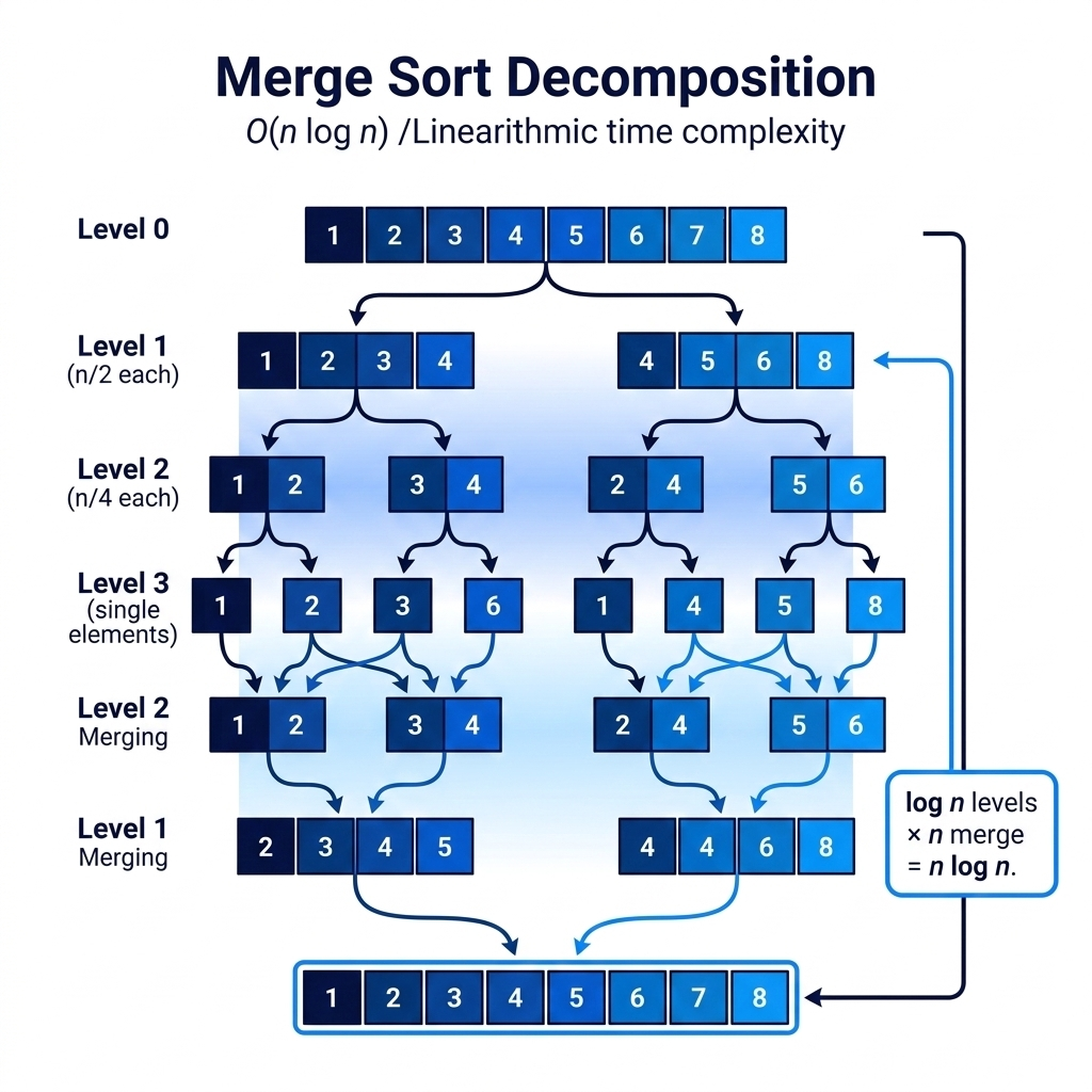
O(n log n) is the complexity class where most efficient sorting algorithms live, and it represents a kind of natural ceiling for comparison-based sorting. It's provably impossible to sort an arbitrary list of n items by comparing elements faster than O(n log n) in the general case — you'd need additional information about the data (like knowing values fall in a fixed range) to do better.

Merge sort is the classic example. The algorithm splits an array in half recursively (the log n part — you can only halve a collection log n times before reaching individual elements), then merges the sorted halves back together (the n part — merging takes linear time). The result is a guaranteed O(n log n) sort in all cases — best, worst, and average. Quick sort also achieves O(n log n) on average, though it degrades to O(n²) in the worst case (which is why it needs careful pivot selection or randomization in production implementations).

# Merge sort — O(n log n) guaranteed
def merge_sort(arr):
    if len(arr) <= 1:
        return arr  # base case

    mid = len(arr) // 2
    left = merge_sort(arr[:mid])   # O(log n) recursive splits
    right = merge_sort(arr[mid:])  # O(log n) recursive splits

    return merge(left, right)       # O(n) merge at each level

def merge(left, right):
    result = []
    i = j = 0
    while i < len(left) and j < len(right):
        if left[i] <= right[j]:
            result.append(left[i])
            i += 1
        else:
            result.append(right[j])
            j += 1
    return result + left[i:] + right[j:]

# Python's built-in sort uses Timsort — also O(n log n), but optimized
# for real-world data patterns (partially sorted arrays, etc.)
data = [38, 27, 43, 3, 9, 82, 10]
print(merge_sort(data))  # [3, 9, 10, 27, 38, 43, 82]

The practical takeaway for everyday engineering: if you find yourself writing a nested loop to sort data or a custom sorting routine, stop. Python's sorted(), JavaScript's .sort(), and equivalents in most languages are implemented in optimized O(n log n) algorithms tuned by compiler engineers over decades. Use them. Your hand-rolled sort is almost certainly slower in practice even if the Big O class is the same.

Pro Tips & Common Mistakes — O(n log n)

Pro Tip: If you need to sort a collection and then immediately binary search it, the total complexity is O(n log n) + O(log n) = O(n log n). The sort dominates. But if you're going to search the same sorted collection hundreds of times, the one-time sort cost amortizes to near-zero per search. Sort once, search many — it's almost always worth it.

Common Mistake: Assuming O(n log n) is "good enough" for all sorting needs. For very small arrays (under ~10 elements), insertion sort (O(n²)) actually outperforms merge sort because of lower overhead and better cache behavior. This is why most production sort implementations switch to insertion sort for small subarrays. Python's Timsort does exactly this.

O(n²) and Beyond: The Danger Zone 

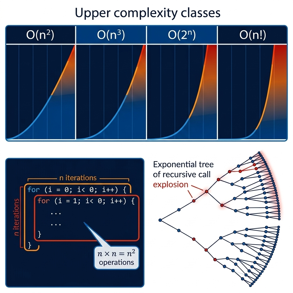
This is where algorithms stop scaling and start breaking production systems. O(n²), O(n³), O(2^n), and O(n!) are the complexity classes where what works in testing collapses under real data — and where that junior engineer's nested loop was sitting quietly, waiting to cause a 2 a.m. incident.

O(n²) — Quadratic Time is the first "danger zone" class. The hallmark is nested loops, both iterating over the same data. Bubble sort is the textbook example: for each of n elements, compare it to every other element — n × n = n² operations. At n=1,000, that's 1 million operations. At n=10,000, that's 100 million. At n=100,000, that's 10 billion. The growth is brutal.

# O(n²) — bubble sort (educational only — never use in production)
def bubble_sort(arr):
    n = len(arr)
    for i in range(n):           # outer loop: n iterations
        for j in range(n - i - 1):  # inner loop: up to n iterations
            if arr[j] > arr[j + 1]:
                arr[j], arr[j + 1] = arr[j + 1], arr[j]
    return arr

# The classic accidental O(n²) pattern in real code:
def find_duplicates_slow(items):
    duplicates = []
    for i in range(len(items)):          # O(n)
        for j in range(i + 1, len(items)):  # O(n) nested
            if items[i] == items[j]:
                duplicates.append(items[i])
    return duplicates  # O(n²) total — dangerous at scale

# O(n) fix using a hash set:
def find_duplicates_fast(items):
    seen = set()
    duplicates = set()
    for item in items:            # O(n) single pass
        if item in seen:          # O(1) set lookup
            duplicates.add(item)
        seen.add(item)
    return list(duplicates)       # O(n) total — safe at any scale

O(n³) — Cubic Time shows up in naive matrix multiplication, certain dynamic programming solutions, and some graph algorithms. At n=100, you're doing a million operations. At n=1,000, a billion. Reserved for small, fixed-size inputs where correctness matters more than speed (like a 4x4 transformation matrix in graphics rendering).

O(2^n) — Exponential Time doubles with every additional input element. The canonical example is the naive recursive solution to the Fibonacci sequence without memoization: fib(n) calls fib(n-1) and fib(n-2), each of which calls two more, creating an explosion of redundant computations. Most brute-force solutions to NP-complete problems (like the traveling salesman problem) are exponential. At n=30, that's over a billion operations.

O(n!) — Factorial Time is the theoretical ceiling of impractical. Finding every possible permutation of a set is O(n!). For n=10, that's 3.6 million permutations — manageable. For n=20, that's 2.4 quintillion. For n=30, it's a number with 32 digits. If you encounter an algorithm requiring O(n!) computation on variable-sized input, you've found something that fundamentally cannot scale, and the solution requires a different algorithmic approach — approximation, heuristics, or a smarter mathematical insight.

Pro Tips & Common Mistakes — O(n²) and Beyond

Pro Tip: When you see a nested loop in a code review, don't immediately reject it. Ask: are both loops always iterating over inputs of size n? Or is the inner loop bounded by a small constant? for i in range(n): for j in range(8): is O(8n) = O(n), not O(n²). The danger is when both loops scale with the same input.

Common Mistake: Using O(2^n) recursive solutions in production without memoization. The classic is Fibonacci: def fib(n): return fib(n-1) + fib(n-2). Without caching intermediate results, this makes an astronomically redundant number of calls. Add @functools.lru_cache in Python or implement a memoization map, and you reduce it to O(n). This is called dynamic programming — and it's one of the most powerful complexity-reduction techniques available.

The Hardware Truth: Why Big O Is Only Half the Story 

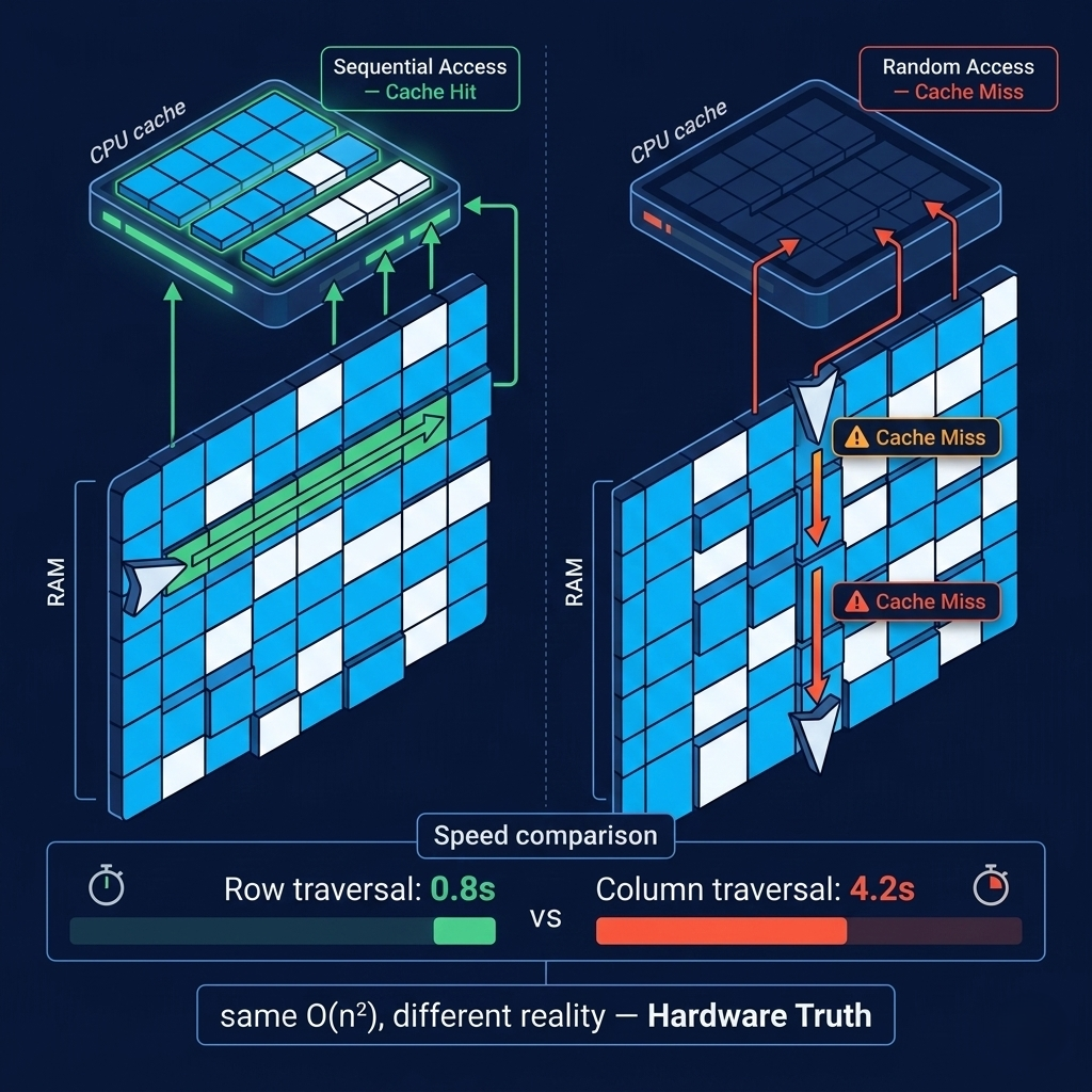
Here's the counterintuitive insight that separates senior engineers from engineers who are technically correct but mysteriously slow in production: two algorithms with identical Big O complexity can have a performance difference of 10x or more in practice, purely based on how they interact with your hardware.

The culprit is cache locality — the principle that CPUs can access data already in their cache (L1, L2, L3) dramatically faster than data that has to be fetched from main memory. We're talking nanoseconds versus hundreds of nanoseconds. An L1 cache hit takes ~1ns. A RAM access takes ~100ns. That's a 100x difference, and it completely dwarfs algorithmic constant factors at the scale of millions of operations.

Consider traversing a 2D array. If you loop row-by-row (arr[row][col]), you access memory in order — each element sits adjacent to the next in RAM. The CPU's prefetcher loads ahead, and almost every access is a cache hit. If you loop column-by-column (arr[col][row]), you jump across memory with every step — each new column access is in a completely different memory region. Cache misses dominate. The difference in runtime for a large 2D array traversal can be 3–10x, even though both are O(n²) in Big O terms.

import time

# Demonstrating cache locality effect
SIZE = 2000
matrix = [[i * SIZE + j for j in range(SIZE)] for i in range(SIZE)]

# Row-major traversal (cache-friendly — sequential memory access)
start = time.time()
total = 0
for row in range(SIZE):
    for col in range(SIZE):      # accesses arr[0][0], arr[0][1], arr[0][2]...
        total += matrix[row][col]  # sequential — cache-friendly
row_time = time.time() - start

# Column-major traversal (cache-unfriendly — random memory jumps)
start = time.time()
total = 0
for col in range(SIZE):
    for row in range(SIZE):      # accesses arr[0][0], arr[1][0], arr[2][0]...
        total += matrix[row][col]  # jumping — cache-unfriendly
col_time = time.time() - start

print(f"Row-major: {row_time:.3f}s")     # typically ~0.8s
print(f"Column-major: {col_time:.3f}s")  # typically ~3-5s on same hardware
# Same Big O (n²). Different hardware behavior. Real performance difference.

The arrays-versus-linked-lists story tells the same tale. Both offer O(n) traversal in Big O notation. But arrays store elements contiguously in memory — the cache loads a whole chunk of adjacent elements at once, and walking through the array is blazing fast. Linked list nodes are scattered across the heap wherever the allocator put them. Walking a linked list means chasing pointers across random memory addresses — each step is potentially a cache miss. For sequential traversal of large datasets, arrays can be 5–10x faster than linked lists in practice despite having the same theoretical complexity.

Pro Tips & Common Mistakes — Hardware Reality

Pro Tip: When working with large collections that you'll traverse frequently, prefer arrays (Python lists, NumPy arrays, Java ArrayLists) over pointer-based structures (Python custom linked lists, Java LinkedList). The cache locality difference is real and measurable. For insertions/deletions in the middle, linked lists win on algorithmic complexity — but even then, the cache penalty often makes arrays faster in practice for reasonably-sized data.

Common Mistake: Optimizing Big O while ignoring memory layout. A developer might replace an O(n²) algorithm with an O(n log n) one but inadvertently introduce scattered heap allocations that destroy cache performance. Always profile. The perf tool on Linux, Instruments on macOS, or cProfile in Python will show you where time is actually being spent — and it's often not where theory says it should be.

How It All Connects: Reading Complexity Like a Senior Engineer 

Let's step back and see the whole picture. Big O is not a checklist of algorithms to memorize — it's a way of thinking about problems and solutions.

When a senior engineer looks at code, they're running a continuous background process: what's the complexity of this, and is that appropriate for how it's used? A triple-nested loop processing a config file with 12 entries is fine — O(n³) at n=12 is 1,728 operations, which is nothing. The same loop processing user-generated content where n could be 100,000 is a disaster waiting to happen. Context is everything. Scale is everything.

The hierarchy from O(1) to O(n!) is a spectrum of scaling behavior, not a moral ranking. O(1) is ideal but impossible for many problems. O(log n) requires sorted or tree-organized data. O(n) is unavoidable whenever you must process every input. O(n log n) is the price of sorting. O(n²) is often a signal to look for a hash map or a smarter algorithm — but not always. And O(2^n) or O(n!) are signals to use approximation, heuristics, or dynamic programming.

The hardware layer — caches, memory layout, branch prediction — is the layer where theory meets reality. Two algorithms at O(n) can behave like O(n) and O(10n) in practice because of how they access memory. Profile your critical paths, measure instead of assuming, and let real numbers guide your optimizations. Big O tells you the shape; profiling tells you the size.

Getting Started: Analyzing Your Own Code 

Here's a practical workflow for applying Big O thinking to your actual codebase, not just toy examples.

Step 1: Identify your input variable

What is n? For most functions, it's obvious: the length of the array, the number of database records, the size of the file. For some functions it's less clear — a function that takes two arrays of different sizes has two variables (n and m), and complexity might be O(n × m), not O(n²).

Step 2: Count your loops

def analyze_me(data):
    result = {}

    for item in data:                    # O(n) — one loop
        result[item] = item * 2          # O(1) — hash set operation

    sorted_data = sorted(data)           # O(n log n) — built-in sort

    for i, item in enumerate(sorted_data):   # O(n) — another loop
        if item in result:                   # O(1) — dict lookup
            sorted_data[i] = result[item]

    return sorted_data

# Analysis:
# First loop: O(n)
# Sort: O(n log n)  ← dominates
# Second loop: O(n)
# Total: O(n) + O(n log n) + O(n) = O(n log n)

Step 3: Identify the dominant term

Drop constants and lower-order terms. O(n log n + n + 50) simplifies to O(n log n). The dominant term is what grows fastest and therefore controls behavior at scale.

Step 4: Look for hidden O(n) operations inside loops

# This looks like O(n) but is actually O(n²)
def hidden_quadratic(data):
    for item in data:                    # O(n) outer loop
        if item in data:                 # O(n) — list 'in' is a scan!
            print(item)
# Fix: convert data to a set before the loop
data_set = set(data)
for item in data:
    if item in data_set:                 # O(1) — now truly O(n) total
        print(item)

Step 5: Profile before optimizing

# Python profiling — find where your code actually spends time
python -m cProfile -s cumulative my_script.py

# For line-by-line profiling, install line_profiler
pip install line_profiler
kernprof -l -v my_script.py  # add @profile decorator to target functions

Step 6: Measure the impact of your changes

import timeit

# Compare two approaches with realistic input sizes
def approach_one(data):
    return [item for item in data if item in data]  # O(n²)

def approach_two(data):
    data_set = set(data)
    return [item for item in data if item in data_set]  # O(n)

data = list(range(10_000))

time_one = timeit.timeit(lambda: approach_one(data), number=10)
time_two = timeit.timeit(lambda: approach_two(data), number=10)

print(f"O(n²) approach: {time_one:.3f}s")   # e.g. 8.2s
print(f"O(n) approach:  {time_two:.3f}s")   # e.g. 0.01s
# Same logical result. 820x speed difference.

FAQ 

Q: Do I need to know Big O Notation for a programming job?

Yes, and not just for interviews. Understanding complexity shapes how you design systems, write code reviews, and debug performance problems. Interview questions exist because Big O is genuinely useful, not as arbitrary gatekeeping. That said, you don't need to memorize every obscure data structure — fluency with O(1), O(log n), O(n), and O(n²) covers the vast majority of real-world decisions.

Q: What's the difference between time complexity and space complexity?

Time complexity measures how the runtime scales with input size. Space complexity measures how the memory usage scales with input size. An algorithm can be O(n) in time and O(1) in space (iterative single pass, no extra memory) or O(n) in both (storing results proportional to input). The notation is the same; the resource being measured is different. Both matter in production, especially when memory is constrained (mobile apps, embedded systems, serverless with small memory limits).

Q: Is O(n log n) always better than O(n²)?

For large n, yes. For small n, not necessarily. At n=5, an O(n²) algorithm does 25 operations; an O(n log n) algorithm does about 12. But if the O(n log n) algorithm has high constant overhead (complex merging logic, function call overhead), it might actually be slower in wall time. Python's sort switches to insertion sort (O(n²)) for arrays smaller than 64 elements precisely because the practical speed is better despite worse theoretical complexity.

Q: What is amortized complexity?

Amortized complexity is the average cost per operation over a sequence of operations, even if individual operations are occasionally expensive. Python lists (dynamic arrays) are a classic example: appending to a list is O(1) on average, but occasionally triggers an O(n) resize when the internal buffer fills. Because resizes happen exponentially less frequently as the list grows, the amortized cost per append is O(1). This is why append() is fast in practice even though it occasionally does a lot of work.

Q: How does Big O relate to database query performance?

Almost directly. A table scan (no index) is O(n) — reads every row. An indexed lookup using a B-tree is O(log n) — follows the tree to the target. A join between two unsorted tables can be O(n × m) — quadratic with table sizes. Understanding this is why adding the right index transforms a slow query into a fast one: you're changing the algorithm's complexity class from O(n) to O(log n).

Q: What does "O(1) amortized" mean for hash tables?

Hash table lookups, insertions, and deletions are O(1) amortized. In the average case, hashing the key and accessing the bucket is constant time. But if the hash table becomes too full (high load factor), it triggers a rehash — rebuilding the entire table at O(n) cost. Because rehashing happens rarely and the table doubles in size each time, the amortized cost per operation remains O(1). Java's HashMap rehashes at 75% capacity by default; Python's dict at approximately 67%.

Q: Can an algorithm be O(n) in Big O but still be too slow?

Absolutely. Big O drops constants, but constants matter in practice. An O(n) algorithm with a constant of 10,000 (doing 10,000 operations per element) might be slower than an O(n²) algorithm with a constant of 0.001 for the sizes of n you're actually working with. This is why "profile first, optimize second" is the right order. Big O tells you how an algorithm scales eventually. Profiling tells you how it performs now on your actual data.

Q: What's the best Big O to aim for when writing code?

Write correct code first. Then measure. Then optimize if needed. In practice, most application code doesn't need to go below O(n log n) — and much of it is fine at O(n). Focus your complexity optimization efforts on the hot paths: database queries, data processing functions called thousands of times per request, and algorithms operating on large user-generated datasets. An O(n²) algorithm called once during server startup processing 20 items is irrelevant. The same algorithm processing every incoming API request at n=50,000 is a production incident waiting to happen.

Conclusion 

Big O Notation is the engineering discipline of thinking ahead. It's the difference between code that embarrasses you six months after launch and code that handles 10x growth without a rewrite. And despite how it's often taught — as a series of notations to memorize for whiteboard interviews — it's actually a practical, daily-use thinking tool.

The hierarchy runs from O(1) at the speed of hardware to O(n!) at the edge of theoretical impossibility. Most real-world engineering decisions live in the middle: understanding when your O(n) scan should be replaced by an O(log n) index, recognizing when a nested loop is an accidental O(n²), and knowing that sometimes the "worse" algorithm is actually faster because of cache behavior your Big O analysis doesn't capture.

The final lesson: Big O is the map, but profiling is the territory. Use complexity analysis to design better algorithms and catch scaling problems before they reach production. Then measure the actual performance — because hardware, cache, memory layout, and constant factors write the final chapter of every performance story.